Baron Services DSSR-250C Pulsar Digital Solid-State Radar System User Manual

Baron Services Inc Pulsar Digital Solid-State Radar System

UserManual.wiki >

Baron Services >

DSSR-250C User Manual >

Processing Algorithms HTML Version

Processing Algorithms

RVP8 User’s Manual

March 2006

5–1

5. Processing Algorithms

Note: Optional dual polarization processing algorithms are described in Appendix B.

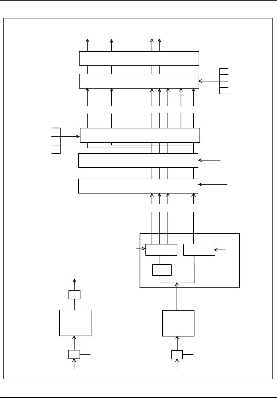
This chapter describes the processing algorithms implemented within the RVP8 signal processor.

The discussion is confined to the mathematical description of these algorithms. Figure 5–1

shows the overall process by which the RVP8 converts the IF signal into corrected reflectivity,

velocity, and width. Table 5–1 summarizes the quantities that are measured and computed by the

RVP8. The type of the quantity (i.e., real or complex) is also given. Subscripts are sometimes

used to denote successive samples in time from a given range bin. For example, sn denotes the

“I” and “Q” time series or “video” sample from the n’th pulse from a given range bin. In cases

where it is obvious, the subscripts denoting the pulse (time) are dropped. The descriptions of all

the data processing algorithms are phrased in terms of the operations performed on data from a

single range bin- identical processing then being applied to all of the selected ranges. Thus, there

is no need to include a range subscript in this data notation.

It is frequently convenient to combine two simultaneous samples of “I” and “Q” into a single

complex number (called a phaser) of the form:

s+I)jQ

where “j” is the square root of –1. Most of the algorithms presented in this chapter are defined in

terms of the operations performed on the “s”’s, rather than the “I”’s and “Q”’s. The use of the

complex terms leads to a more concise mathematical expression of the signal processing

techniques being used. In actual operation, the complex arithmetic is simply broken down into

its real-valued component parts in order to be computed by the RVP8 hardware. For example,

the complex product:

s+W Y

is computed as

Real{s}+Real{W}Real{Y}*Imag{W}Imag{Y}

Imag{s}+Real{W}Imag{Y})Imag{W}Real{Y}

where “Real{}” and “Imag{}” represent the real and imaginary parts of their complex-valued

argument. Note that all of the expanded computations are themselves real-valued.

In addition to the usual operations of addition, subtraction, division, and multiplication of

complex numbers, we employ three additional unary operators: “||”, “Arg” and “*”. Given a

number “s” in the complex plane, the magnitude (or modulus) of s is equal to the length of the

vector joining the origin with “s”, i.e. by Pythagoras:

|s|+Real{s}2)Imag{s}2

The signed (CCW positive) angle made between the positive real axis and the above vector is:

ë+Arg{s}+arctanƪImag{s}

Real{s}ƫ

Processing Algorithms

RVP8 User’s Manual

March 2006

5–2

where this angle lies between *p and )p and the signs of Real{s} and Imag {s} determine

the proper quadrant. Note that this angle is real, and is uniquely defined as long as |s| is

non-zero. When |s| is equal to zero, Arg{s} is undefined. Finally, the “complex conjugate” of “s”

is that value obtained by negating the imaginary part of the number, i.e.,

s*+Real{s}*jImag

{s}.

Note that Arg{s*} = –Arg{s}. The reader is referred to any introductory text on complex

numbers for clarification of these points.

Table 5–1: Algebraic Quantities Within the RVP8 Processor

pInstantaneous IF-receiver data sample Real

bInstantaneous Burst-pulse data sample Real

I,QInstantaneous quadrature receiver components Real

s Instantaneous time series phaser value Complex

sȀTime series after clutter filter Complex

T0Zeroth lag autocorrelation of A values Real

R0Zeroth lag autocorrelation of AȀ values Real

R1First lag autocorrelation of AȀ values Complex

R2Second lag autocorrelation of AȀ values Complex

SQI Signal Quality Index Real

V Mean velocity Real

W Spectrum Width Real

CCOR Clutter correction Real

LOG (Signal+Noise)/Noise ratio for thresholding Real

SIG Signal power of weather Real

C Clutter power Real

N Noise power Real

ZCorrected Reflectivity factor Real

TUnCorrected Reflectivity factor Real

The following sections cover the various parts of the diagram shown in Figure 5–1, i.e.,

SIF Signal Processing

SI/Q processing and clutter filtering

SRange averaging and clutter microsuppression

SMoment calculations (reflectivity, velocity, spectrum width)

SThresholding for data quality and Speckle Filtering

SReflectivity Calibration

SSpecial algorithms for ambiguity resolution (dual PRF, dual PRT, Random Phase)

SCalibration and Testing

Processing Algorithms

RVP8 User’s Manual

March 2006

5–3

Speckle Remover

Thresholding

Calibrate Moments

Range Averaging

Micro Clutter Suppression

dBZ dBT V W

V W SQI SIG CCOR

SIGTH

LOGTH

SQITH

CCORTH

FLAGS

dBZ dBT

K–bins

dBZ0

CCORTH

Correlate Correlate

Filter

R0 R1 (R2) T0

36 MHz

Figure 5–1: Flow Diagram of RVP8 Processing

Calculate Output Data

FIR

Decimate

in Time

A/D

36 MHz

Burst IF Input Channel

FFT

Compute

Frequency

A/D

D/A

AFC

(I and Q)

Clutter Filtering and Autocorrelation by

Time Domain or Frequency Domain Approach

IF Signal Input Channel

Processing Algorithms

RVP8 User’s Manual

March 2006

5–4

5.1 IF Signal Processing

The starting point for all computations within the RVP8 are the instantaneous IF-receiver

samples pn and, the instantaneous burst-pulse or COHO reference samples bn. These data are

available at a very high sampling rate (typically 36MHz), which makes possible the digital

implementation of functions that are traditionally performed by discrete components in an

analog receiver. The RVP8’s all-digital approach replaces a great deal of analog hardware,

avoids problems of aging and maintenance, and makes it easy to tune-up the receiver and alter

its parameters.

This section describes these IF signal processing steps. Please refer to Figure 1-3 for a block

diagram of the IF processing that is performed.

5.1.1 FIR (Matched) Filter

The RVP8 implements a digital version of the “matched” filter that is found in the traditional

analog radar receiver. The equivalent Finite-Impulse-Response (FIR) filter is designed using an

interactive graphical procedure described in Section 4.4. The filter length (number of taps),

center frequency, and bandwidth are all adjustable. The design procedure computes two sets of

filter coefficients fin and fqn such that the instantaneous quadrature samples at a given bin are:

I+ȍ

N*1

n+0

fin pn,Q+ȍ

N*1

n+0

fqn pn

where N is the length of the filter. The input samples pn are centered on the range bin to which

the (I,Q) pair is assigned. Note that some of the pn are likely to overlap among adjacent bins,

i.e., the filter length may be chosen to be greater than the bin spacing. Such an overlap

introduces a slight correlation between successive bins, but the longer length allows a better

filter to be designed.

The sums above for I and Q are computed on the RVP8/Rx board using dedicated FIR chips (for

revisions A and B) that can perform up to 576 million sums of products per second. The Rev C

RVP8/Rx uses a more flexible FPGA. The pn are represented as 16-bit signed integers, and the

fin and fqn are represented as 10-bit (Rev.A/B) or 16-bit (Rev.C) signed integers. A numerical

optimization procedure is used to quantize the ideal filter coefficients into their hardware values.

The overall spectral purity of the FIR filter will typically be greater than 66dBc (Rev.A/B) and

84dBc (Rev.C).

The reference phase for each transmitted pulse is computed using the same two FIR sums,

except with bn substituted for the pn. For a magnetron system the Nb

n samples are centered

on the transmitted burst; for a Klystron system they may be obtained from the burst pulse

(recommended) or from the CW COHO. If the Klystron is phase modulated by an external

phase shifter (as opposed to the RVP8/Tx digital transmitter board), then the samples should be

from the modulated COHO.

The fin coefficients are computed as:

fin+ln sinƪp

4)2pfIF

fSAMP ǒn*N*1

2Ǔƫ,n+0AAA N*1

Processing Algorithms

RVP8 User’s Manual

March 2006

5–5

where fIF is the radar intermediate frequency, fSAMP is the RVP8/IFD crystal sampling

frequency, and ln are the coefficients of an N-point symmetric low-pass FIR filter that is

matched to the bandwidth of the transmitted pulse. The multiplication of the ln terms by the

sin() terms effectively converts to the low-pass filter to a band-pass filter centered at the radar IF.

The formula for the fqn coefficients is identical except that sin() is replaced with cos().

The phase of the sinusoid terms, and the symmetry of the ln terms, has been carefully chosen to

have a valuable overall symmetry property when n is replaced with (N–1)–n, i.e., the sequence is

reversed:

fi(N*1)*n+l(N*1)*n sinƪp

4)2pfIF

fSAMP ǒ((N*1) *n)*N*1

2Ǔƫ

fi(N*1)*n+ln cosƪp

4)2pfIF

fSAMP ǒn*N*1

2Ǔƫ

fi(N*1)*n+fqn

Thus, the coefficients needed to compute I are merely the reversal of the coefficients needed to

compute Q; if you know fin, then you also know fqn.

5.1.2 RVP8/Rx Receiver Modes

The RVP8 supports six fundamental IFD and RVP8/Rx configurations which allow you to

choose the best style of IF processing for your particular site. The following table summarizes

the options where, BW is the net IF sampling rate (full 72MHz, or halfband filtered 36MHz),

DynR is the dynamic range (normal single channel, or extra wide dual channel), Pol is the

number of polarizations, Freq is the number of distinct intermediate frequencies, and IFD is the

number of IFD’s, along with their corresponding RVP8/Rx cards.

# BW DynR Filt Pol Freq IFD Description

– –––– –––– –––– ––– –––– ––– ––––––––––––––––––––––

0 Full Norm Norm 1 1 1 Standard single channel

1 Full Norm Norm 2 2 1 Dual Pol on two frequencies

2 Full Norm Norm 2 1 2 Dual Pol on separate IFDs

3 Half Norm Norm 2 1 1 Dual Pol on single IFD

4 Half Wide Norm 1 1 1 Extra wide dynamic range

5 Half Norm Long 1 1 1 Extra long/fast FIR filters

The first three modes were already supported in the previous RVP7 processor. The last three

modes are unique to the RVP8 and bring some exciting additional capabilities to the signal

processor. The six receiver modes are summarized below. Please see the Discussion of

Halfband Filtering (Section 5.1.2.1) as it applies to Modes 3-5, and the Discussion of Wide

Dynamic Range (Section 5.1.2.2)for additional details on using Mode-4.

Mode-0: Standard Single Channel This is the most common “vanilla” mode that is used by

single-polarization CW-pulsed radars whose front-end LNA has a dynamic range less than

92dB. The (I,Q) data are computed from IF samples at their full acquisition rate (32MHz for

Rev.D IFDs, and 72MHz for Rev.F), and the resulting dynamic range from 14-bit IFD samples is

well matched to the RF components.

Processing Algorithms

RVP8 User’s Manual

March 2006

5–6

Mode-1: Dual-Pol On Two Frequencies This was the original dual-Pol configuration used by

the RVP7 several years ago. A single IFD A/D converter receives the “H” and “V” channels

using two distinct intermediate frequencies. Two different STALOs are required in this

configuration, making the RF/IF components a bit more expensive, but only one IFD is required.

Mode-2: Dual-Pol On Separate IFDs This mode was introduced into the RVP8 in 2003, and

provides dual polarization data using two IFDs connected to two RVP8/Rx cards in the same PCI

chassis. A single intermediate frequency is used, hence only one STALO is required.

Mode-3: Dual-Pol On Single IFD This is the recommended dual polarization mode for all new

RVP8 installations. The “H” and “V” channels are fed into the Primary and Secondary IFD

inputs using a single intermediate frequency. System cost and complexity are both optimized in

this design since only a single IFD, RVP8/Rx card, and STALO are required to process both

polarization channels.

Mode-4: Extra Wide Dynamic Range Radars having very high performance front-end LNAs

can preserve the full benefit of that investment by running two separate IF signals into the

Primary (HiGain) and Secondary (LoGain) IFD inputs. A nominal channel separation of

25–30dB might be used to achieve an overall dynamic range of up to 110dB.

Mode-5: Extra Long/Fast FIR Filters This mode is intended for pulse compression systems

that require unusually long filters (up to 80μsec), or finer range resolution in order to employ

higher compressed bandwidths without the risk of missing echoes between bins. For example, a

30μsec pulse could be processed at an incoming range resolution of 50 meters and then range

averaged down to 150meter output spacing.

5.1.2.1 Discussion of Halfband Filtering Modes 3-5

Traditionally, the IFD used by the RVP7 and RVP8 has sent raw 14-bit A/D samples from

its Burst and IF inputs directly to either the RVP7/Main or RVP8/Rx cards for FIR filtering

and conversion into complex (I,Q) values. The IFD would function simply as a waveform

sampling device (hence the acronym IF Digitizer), and all of the front-end signal processing

took place downstream of it.

This model has changed with the introduction of the Rev.F IFD which has the ability to carry

out several billion multiply-accumulate cycles per second. This means that IF samples from

multiple signals can be preprocessed entirely within the IFD and then encoded without loss

onto the fixed bandwidth of its digital downlink. The new receiver modes 3 through 5 rely

on this hardware capability and use a method known as “Halfband Filtering” to effectively

double the downlink data rate.

Section 2.2.7 of the RVP8 User’s Manual contains a detailed account of how A/D quantiza-

tion noise affects the dynamic range of the IFD. Briefly, for the Rev.F A/D converter which

runs at 72MHz, the contribution of A/D quantization noise within any given 1MHz interval

is 72 times smaller than the total noise of the converter itself. This is an important property

of all wideband sampling systems: the noise floor after processing, and hence the dynamic

range, are improved by increasing the fundamental A/D sampling rate.

Normally the IFD sends 72MHz A/D samples from a single input channel directly down to

the RVP8/Rx PCI card. The samples are sent at full speed in order to realize maximum reduc-

Processing Algorithms

RVP8 User’s Manual

March 2006

5–7

tion of the final (I,Q) noise floor. But suppose we wanted to send two A/D waveforms down

the same data link by interleaving the samples together. Each channel would have to be

down-sampled to 36MHz in order to fit within this format, but that would cause its (I,Q)

noise floor to increase by 3dB.

To avoid this, we do not create the 36MHz streams merely by discarding every other A/D

sample, but rather, by passing the original 72MHz data through a halfband digital filter and

then discarding every other point of this filtered A/D stream. The difference is important.

Since the halfband filter has removed all of the A/D quantization noise from half of the origi-

nal Nyquist interval, there will be no increase in noise density within the passband of the

(I,Q) filter when the halfband stream is down sampled to 36MHz. Thus, the A/D noise that

would normally have folded into the (I,Q) data at 36MHz is first removed by the halfband

filter so that we’re left with a 36MHz stream having the same dynamic range of the original

72MHz samples.

The IFD halfband filter is a 49-Tap equiripple FIR filter having 40dB of stopband rejection

and 0.175dB of passband ripple. The passband extends either from 0–16.5MHz when con-

figured as a lowpass filter, or 19.5–36MHz when configured for highpass. The RVP8 auto-

matically selects the correct type of filter depending on the intermediate frequency specified

in the Mb menu. The halfband filter has linear phase and is therefore non-dispersive. This

means that it is totally suitable for handling compressed pulses and other wideband Tx/Rx

waveforms.

5.1.2.2 Discussion of Wide Dynamic Range Mode-4

When a two channel IFD is used as an extended dynamic range receiver there are some im-

portant decisions to make with respect to setting up the RF/IF levels that drive the IFD.

The first of these is the amount of signal level separation between the high gain and the low

gain IFD inputs. There is an absolute minimum and absolute maximum channel separation

that still allows the IFD to capture the full dynamic range of the receiver. If a signal level

separation is made that is outside of these absolute limits valuable receiver dynamic range

will be lost.

SThe absolute minimum separation of the channels is equal to the total dynamic

range of the receiver minus the dynamic range of a single channel of the IFD.

Generally, the total dynamic range of the receiver is set by the LNA. For

example, if we are considering a 1μsec pulse (1MHz bandwidth), the dynamic

range of the LNA may be about 105dB, and the dynamic range of a single

channel of the IFD is about 84dB (from –78dBm to +6dBm). In this case, the

minimum separation would be 21dB. At minimum separation, the overlap of the

low gain channel and the high gain channel will be maximized, and that overlap

is equal to the dynamic range of a signal channel of the IFD minus the separation.

In this case, the overlap is ( 84dB – 21dB ) = 63dB.

SThe absolute maximum separation of the channels is simply the dynamic range

of a single channel of the IFD. In the above example this would be 84dB. At

Processing Algorithms

RVP8 User’s Manual

March 2006

5–8

maximum separation, the overlap of the low gain channel and the high gain

channel is zero -- we begin using one as soon as the other has begun to saturate.

We see that there can be a large difference between the absolute minimum and maximum

signal level separations; thus additional criteria must be considered to choose an optimum

value that is between these diverse limits.

Choosing a proper separation value is a tradeoff of several factors. If the separation value

is too low, the IFDs may end up operating very close to their noise floors. And if the separa-

tion is too high, then the overlap between the two channels is reduced which makes it difficult

for the IFD to make a smooth transition as it combines the data from both channels. Too high

a separation may also result in receiver components that are not practical to build.

As a rule of thumb, channel separations in the 22–30dB range provide a good balance of the

above criteria. In the case of a 1μsec pulse this results in an overlap interval of approximately

55-63dB, which is sufficient for good IFD transitions and also leads to receiver components

that are practical to build.

Once a separation value has been chosen, one must consider how to build the receiver to

achieve this. The basic receiver will take the form of an LNA and a mixer followed by a

splitter resulting in a low gain channel and a high gain channel. We know the gain difference

in the two channels (the separation value), but we must find the actual gain to use in each

channel.

If we consider the total system dynamic range as generally set by the LNA (105dB in the

above example), we can estimate the minimum detectable signal input to the LNA as well

as the maximum usable linear level at the IFD. If the LNA has a noise figure of 1dB and

we are using a 1μsec pulse, the minimum detectable signal at the LNA input is –113dBm,

and thus the maximum signal is 105dB above this, or –8dBm. If we add to these number

the gain of the LNA and the conversion loss of the mixer (and any other losses experienced

through the power splitter for the low gain and high gain channels), we can use this informa-

tion to determine the signal values of the components in these two channels.

For example, if the LNA has a gain of 17dB, the mixer has a conversion loss of 7dB, there

is 1dB miscellaneous losses and 3dB loss in the power splitter, then the signal level at the

output of the power splitter is ( –113 + 18 – 7 – 1 – 3 ) = –106dBm for the minimum signal,

and and –1dBm for the maximum signal. In the low gain channel, we need to bring the

–1dBm up to the maximum input value of the IFD (+6dBm). To do this we need about 8dB

of amplification (7dB plus one more deciBel to account for the anti–alias filter loss of the

IFD). If we assume 25dB of channel separation, on the high gain channel we require about

+33dB of amplification. Finally, this tells us that on the low gain channel, the minimum and

maximum signals presented to the IFD are ( –106 + 8 ) = –98dBm and ( –1 + 8 ) = 7dBm.

For the high gain channel, the signal levels are ( –106 + 33 ) = –73dBm and ( –1 + 33 ) =

+32dBm. Note that as +32dBm is above the maximum input level tolerated by the IFD, the

amplifier on the high gain channel must limit its output to less than +16dBm. Thus an ampli-

fier with an output saturation value of between +10dBm and +15dBm should be used.

Processing Algorithms

RVP8 User’s Manual

March 2006

5–9

5.1.3 Automatic Frequency Control (AFC)

AFC is used on magnetron systems to tune the STALO to compensate for magnetron frequency

drift. It is not required for Klystron systems. The STALO is typically tuned 30 or 60 MHz away

from the magnetron frequency. The maximum tuning range of the AFC feedback is

approximately 7MHz on each side of the center frequency. This is limited by the analog filters

that are installed just before the signal and burst IF inputs on the IFD. It is important that the

system’s IF frequency is at least 4MHz away from any multiple of half the digital sampling

frequency, i.e., 18, 36, 54, or 72MHz.

The RVP8 analyzes the burst pulse samples from each pulse, and produces a running estimate of

the power-weighted center frequency of the transmitted waveform. This frequency estimate is

the basis of the RVP8’s AFC feedback loop, whose purpose is to maintain a fixed intermediate

frequency from the radar receiver.

The instantaneous frequency estimate is computed using four autocorrelation lags from each set

of Nb

n samples. This estimate is valid over the entire Nyquist interval (e.g., 18MHz to

36MHz), but becomes noisy within 10% of each end. Since the span of the burst pulse samples

is only approximately one microsecond, several hundred estimates must be averaged together to

get an estimate that is accurate to several kiloHertz. Thus, the AFC feedback loop will typically

have a time constant of several seconds or more.

Most of the burst pulse analysis routines, including the AFC feedback loop, are inhibited from

running immediately after making a pulsewidth change. The center-of-mass calculations are

held off according to the value of Settling time (to 1%) of burst frequency estimator, and the

AFC loop is held off by the Wait time before applying AFC (Mb Section 3.2.6). This prevents

the introduction of transients into the burst analysis algorithms each time the pulsewidth

changes.

Additional information about using AFC can be found in Sections 2.2.11, 2.4, and 3.2.6.

5.1.4 Burst Pulse Tracking

The RVP8 has the ability to track the power-weighted center-of-mass of the burst pulse, and to

automatically shift the trigger timing so that the pulse remains in the center of the burst analysis

window of the Pb plot. This means that external sources of drift in the timing of the transmitted

pulse (temperature, aging, etc.) will be tracked and nulled out during normal operation; so that

fixed targets will remain fixed in range, and clean Tx phase measurements will always be

available on every pulse.

The Burst Pulse Tracker feedback loop makes changes to the trigger timing in response to the

measured position of the burst. Timing changes will generally be made only when the RVP8 is

not actively acquiring data, in the same way that AFC feedback is held off for similar “quiet”

times. However, if the center-of-mass has drifted more than 1/3 the width of the burst analysis

window, then the timing adjustment will be made right away. Also, there will be an

approximately 5ms interruption in the normal trigger sequence whenever any timing changes are

made.

Processing Algorithms

RVP8 User’s Manual

March 2006

5–10

The Burst Pulse Tracker and AFC feedback loop are each fine-tuning servos that keep the burst

pulse “centered” in time and frequency. These servos have been expanded to include a

combined “Hunt Mode” that will track down a missing burst pulse when we are uncertain of

both its time and frequency. This coarse-tuning mode is especially valuable for initializing the

two fine-tuning servos in radar systems that drift significantly with time and temperature.

When the radar transmitter is On but the burst pulse is missing, it may be because either of the

following have happened:

SIt is misplaced in time, i.e., the Tx pulse is outside of the window displayed in the Pb

plotting command. In this case, the trigger timing needs to be changed in order to bring

the center of the pulse back to the center of the window.

SIt is mistuned in frequency, i.e., the AFC feedback is incorrect and has caused the burst

frequency to fall outside of the passband of the RVP8 anti-alias filters. In this case the

AFC (or DAFC) needs to be changed so that proper tuning is restored.

The Hunt Mode performs a 2-dimensional search in time and frequency to locate the burst;

searching across a +20msec time window, and across the entire AFC span. If a valid Tx pulse

(i.e., meeting the minimum power requirement) can be found anywhere within those intervals

then the Burst Pulse Tracker and AFC loops will be initialized with the time and frequency

values that were discovered. The fine servos then commence running with a good burst signal

starting from those initial points.

Depending on how the hunting process has been configured in the Mb menu, the whole

procedure may take several seconds to complete. The RVP8’s host computer interface remains

completely functional during this time, but any acquired data would certainly be questionable.

GPARM status bits in word #55 indicate when the hunt procedure is running, and whether it has

completed successfully. The BPHUNT (Section 6.26) opcode allows the host computer to

initiate Hunt Mode when it knows or can sense that a burst pulse should be present

5.1.5 Interference Filter

The interference filter is an optional processing step that can be applied to the raw (I,Q) samples

that emerge from the FIR filter chips. The intention of the filter is to remove strong but sporadic

interfering signals that are occasionally received from nearby man-made sources. The technique

relies on the statistics of such interference being noticeably different from that of weather.

For each range bin at which (I,Q) data are available, the interference filter algorithm uses the

received power (in deciBels) from the three most recent pulses:

Pn*2,Pn*1, and Pn

where:

Pn+10 log10ǒI2

n)Q2

nǓ .

If the three pulse powers have the property that:

ŤPn*1*Pn*2ŤtC1 and ŤPn*Pn*1ŤuC2 (Alg.1)

Processing Algorithms

RVP8 User’s Manual

March 2006

5–11

then (In,Qn) is replaced by (In*1,Qn*1) . Here C1 and C2 are constants that can be tuned by

the user to match the type of interference that is anticipated, and the error rates that can be

tolerated. For certain environments it may be the case that good results can be obtained with

C1+C2; but the RVP8 does not force that restriction.

This 3-pulse algorithm is only intended to remove interference that arrives on isolated pulses,

and for which there are at least two clear pulses in between. Interference that tends to arrive in

bursts will not be rejected.

Two variations on the fundamental algorithm are also defined. The CFGINTF command

(Section 6.23) allows you to choose which of these algorithms to use, and to tune the two

threshold constants. You may also do this directly from the Mp setup menu (Section 3.2.2).

ŤPn*1*Pn*2ŤtC1 and Pn*Pn*1uC2 (Alg.2)

ŤPn*1*Pn*2ŤtC1 and Pn*LinAvg(Pn*1,Pn*2)uC2 (Alg.3)

Where LinAvg() denotes the deciBel value of the linear average of the two deciBel powers. The

Alg.2 and Alg.3 algorithms also include the receiver noise level(s) as part of their decision

criteria. Whenever power levels are intercompared in the algorithms, any power that is less than

the noise level is first set equal to that noise level. This makes the filters much more robust and

properly tunable, so that interference is more successfully rejected on top of blank receiver

noise.

Optimum values for C1 and C2 will vary from site to site, but some guidance can be obtained

using numerical simulations. The results shown below were obtained when the algorithms were

applied to realistic weather time series having a spectrum width = 0.1 (Nyquist), SNR = +10dB,

and an intermittent additive interference signal that was 16dB stronger than the weather. The

interference arrived in isolated single pulses with a probability of 2%.

Performance of the three algorithms is summarized in the first three columns of Table 5–2, for

which C1 and C2 have the common value shown. The fourth column also uses Algorithm #3,

but with the value of C1 raised by 2dB. The “Missed” rate is defined as the percentage of

interference points that manage to get through the filtering process without being removed. The

“False” (false alarm) rate is the percentage of non-interference points that are incorrectly

modified when they should have been left alone.

Table 5–2: Algorithm Results for +16dB Interference

Alg.1 Alg.2 Alg.3 Alg.3, C1+=2dB

C1,C2 Missed/False Missed/False Missed/False Missed/False

––––– –––––––––––– –––––––––––– –––––––––––– ––––––––––––

6.0dB 17.8% 10.91% 17.8% 4.06% 17.8% 3.48% 10.3% 4.15%

8.0dB 10.5% 6.57% 10.5% 2.42% 10.4% 1.71% 6.1% 1.92%

9.0dB 8.5% 5.09% 8.5% 1.81% 8.3% 1.16% 5.4% 1.28%

10.0dB 7.3% 4.01% 7.3% 1.42% 7.5% 0.79% 5.4% 0.85%

11.0dB 8.9% 3.14% 8.9% 1.06% 8.3% 0.51% 6.5% 0.54%

12.0dB 11.6% 2.53% 11.6% 0.85% 11.3% 0.33% 9.9% 0.35%

13.0dB 17.0% 2.07% 17.0% 0.67% 16.3% 0.22% 15.3% 0.23%

14.0dB 23.5% 1.70% 23.5% 0.54% 22.4% 0.14% 21.6% 0.15%

16.0dB 39.2% 1.21% 39.2% 0.35% 39.6% 0.06% 38.9% 0.06%

20.0dB 67.3% 0.65% 67.3% 0.14% 72.5% 0.01% 72.4% 0.01%

Processing Algorithms

RVP8 User’s Manual

March 2006

5–12

It is important to minimize both types of errors. If too much interference is missed, then the

filter is not doing an adequate job of cleaning up the received signal. If the false alarm rate is

too high, then background damage is done at all times and the overall signal quality (especially

sub-clutter visibility) may be compromised. We suggest that you try to keep the false alarm rate

fairly low, perhaps below 1%; and then let the missed percentage fall where it may.

To summarize the numerical results in Table 5–2:

SThe “Missed” rates of Alg.1 and Alg.2 are identical, but the “False” rate of Alg.1 is

much higher. Alg.1 clearly does not perform as well for additive interference, but it is

included in the suite for historical reasons.

SThe “Missed” error rate for Alg.3 is nearly identical to that of Alg.2, but Alg.3 has a

significantly lower false alarm rate. This is because of the somewhat improved statistics

that result when the linear mean of Pn*2 and Pn*1 is used in the second comparison,

rather than just Pn*1 by itself. We recommend that Alg.3 generally be chosen in

preference to the other two.

SAlg.3 can be further tuned by allowing the two constants to differ. For example, by

raising C1 slightly above C2 (fourth column), we can trade off a decrease in the

“Missed” rate for an increase in the “False” rate. Lowering C1 would have the opposite

effect.

Keep in mind that optimum tuning will depend on the type of interference you are trying to

remove. In the previous example, where the interfering signal is only 16dB stronger than the

weather, there was a close tradeoff between the “Missed” and “False” error rates. However,

Table 5–3 shows the results that would be obtained if the interference dominates by 26db.

Table 5–3: Algorithm Results for +26dB Interference

Alg.1 Alg.2 Alg.3 Alg.3, C2+=5dB

C1,C2 Missed/False Missed/False Missed/False Missed/False

––––– –––––––––––– –––––––––––– –––––––––––– ––––––––––––

6.0dB 17.8% 10.75% 17.8% 3.95% 17.8% 3.44% 17.8% 0.34%

8.0dB 9.9% 6.48% 9.9% 2.31% 9.9% 1.68% 9.9% 0.15%

9.0dB 7.4% 4.99% 7.4% 1.75% 7.4% 1.14% 7.4% 0.10%

10.0dB 5.9% 3.91% 5.9% 1.36% 5.9% 0.76% 5.9% 0.06%

11.0dB 4.8% 3.06% 4.8% 1.06% 4.8% 0.50% 4.8% 0.04%

12.0dB 3.2% 2.37% 3.2% 0.83% 3.2% 0.33% 3.2% 0.03%

13.0dB 2.6% 1.83% 2.6% 0.62% 2.6% 0.20% 2.8% 0.01%

14.0dB 1.9% 1.45% 1.9% 0.50% 1.9% 0.12% 2.6% 0.01%

16.0dB 1.3% 0.90% 1.3% 0.30% 1.3% 0.05% 5.8% 0.00%

20.0dB 3.1% 0.39% 3.1% 0.12% 2.0% 0.01% 31.5% 0.00%

Notice that we can now re-tune the constants and operate with C1+13dB and C2+18dB

(fourth column); which yields a low 2.8% “Missed” rate, and an extremely low 0.01% false

alarm rate. Since the false alarm rate is (approximately) independent of the interference power,

these filter settings would leave all “clean” weather virtually untouched, i.e., we would have a

very safe filter that is intended only to remove fairly strong interference. Such a filter could be

left running at all times without too much worry about side effects.

Processing Algorithms

RVP8 User’s Manual

March 2006

5–13

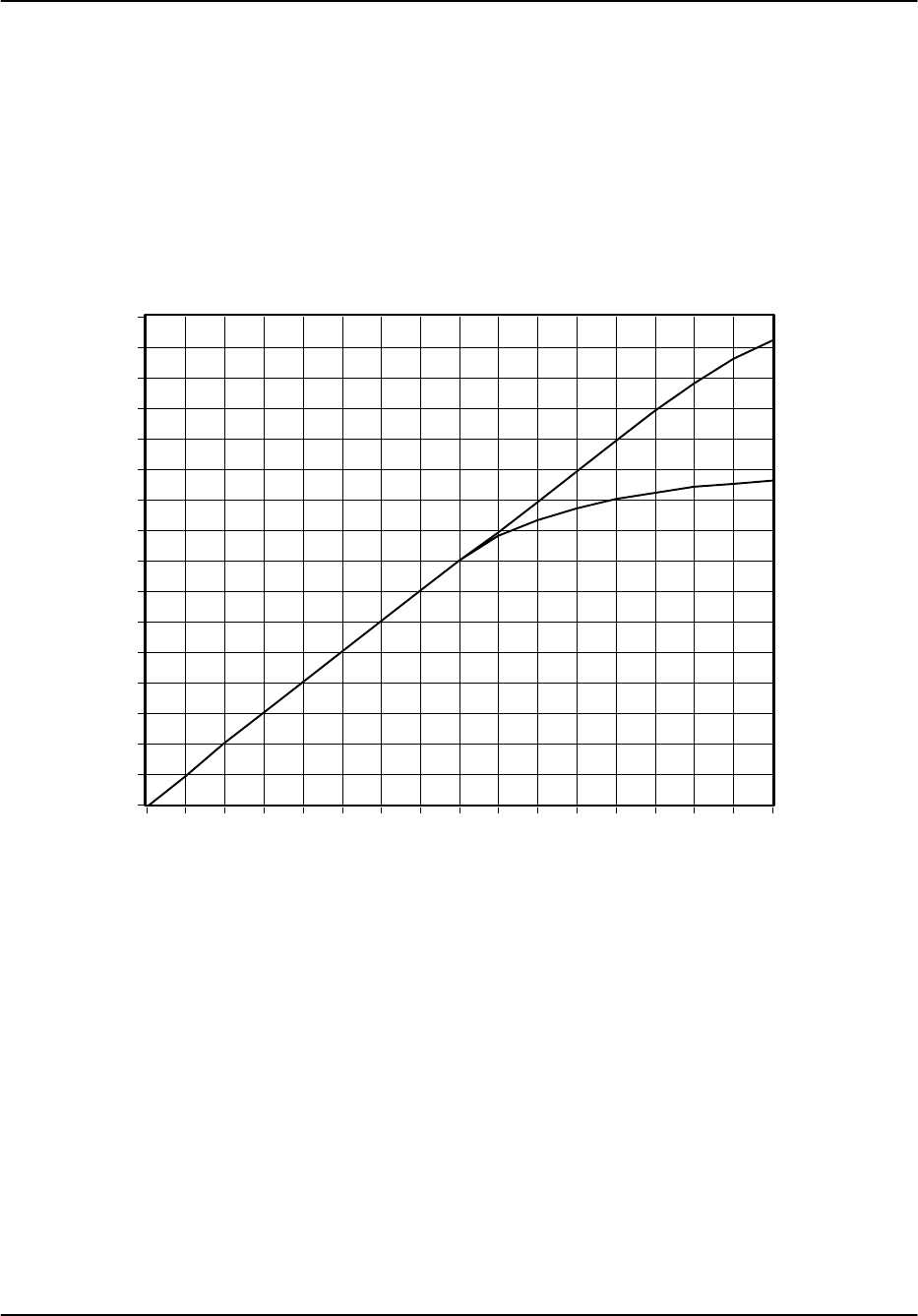
5.1.6 Large-Signal Linearization

The RVP8 is able to recover the signal power of targets that saturate the IF-Input A/D converter

by as much as 4–6 deciBels. This is possible because an overdriven IF waveform still spends

some of its time in the valid range of the converter, and thus, it is still possible to deduce

information about the signal.

Figure 5–2 shows actual signal generator test measurements with normal A/D saturation (lower

line), and with the extrapolation algorithms turned on (upper line). The high-end linear range

begins to roll off at approximately +10dBm versus +5dBm, and thus has been extended by 5dB.

–4

–3

–2

–1

–4–3–2–10123456789101112

Figure 5–2: Linearization of Saturated Signals Above +4.5dBm (Rev B/C IFD)

The roll off starts at +4.5 dBm for the Rev. B&C IFD, and at +6 dBm for the Rev. D.

5.1.7 Correction for Tx Power Fluctuations

The RVP8 can perform pulse-to-pulse amplitude correction of the digital (I,Q) data stream based

on the amplitude of the Burst/COHO input. The technique computes a (real valued) correction

factor at each pulse by dividing the mean amplitude of the burst by the instantaneous amplitude

of the burst. The (I,Q) data for that pulse are then multiplied by this scale factor to obtain

corrected time series. The amplitude correction is applied after the Linearized Saturation

Headroom correction.

The mean burst amplitude is computed by an exponential average whose (1/e) time constant is

selected as a number of pulses (See Section 3.2.2). A short time constant will settle faster, but

will not be as thorough in removing amplitude variations (since the mean itself will be varying).

Processing Algorithms

RVP8 User’s Manual

March 2006

5–14

Longer time constants do a better job, but will require a second or two before valid data is

available when the transmitter is first turned on. The default value of 70 will give excellent

results in almost all cases.

Whenever the RVP8 enters a new internal processing mode (time series, FFT, PPP, etc.), the

burst power estimator is reinitialized from the level of the first pulse encountered, and an

additional pipeline delay is introduced to allow the estimator to completely settle. Thus, valid

corrected data are produced even when the RVP8 is alternating rapidly between different data

acquisition tasks, e.g., in a multi-function ASCOPE display. The additional pipeline delay will

not affect the high-speed performance when the RVP8 runs continuously in any single mode.

For amplitude correction to be applied, the instantaneous Burst/COHO signal level must exceed

the minimum valid burst power specified in the “Mb” setup section. If that level is not met, e.g.,

if the transmitter is turned off, then no correction is performed. Thus, the amplitude correction

feature conveniently “gets out of the way” when receiver-only tests are being performed.

The maximum correction that will ever be applied is 5dB. If the burst power in a given pulse

is more than 5dB above the mean, or less than 5dB below it, then the correction is clamped at

those limits. The power variation of a typical transmitter will easily be contained within this

interval (it is typically less than 0.3dB).

Instantaneous amplitude correction is a unique feature of the RVP8 digital receiver. Bench tests

with a signal generator reveal that an amplitude modulated waveform having 2.0dB of

pulse-to-pulse variation is reduced to less than 0.02dB RMS of (I,Q) variation after applying the

amplitude correction.

Processing Algorithms

RVP8 User’s Manual

March 2006

5–15

5.2 Time Series (“I” and “Q”) Signal Processing

This section describes the processing of the radar time series data (also called linear “video” or

“I” and “Q”) to obtain the meteorologically significant “moment” parameters: reflectivity, total

power, velocity, width, signal quality index, clutter power correction, and optional polarization

variables.

Recall that the time series synthesized by the FIR filter consist of an array of complex numbers:

sm+[Im)jQm]for m+1, 2, 3, AAA,M

where “j” is *11ń2. The time series, are the starting point for all calculations performed

within the RVP8. There are several excellent references on the details of I and Q processing. The

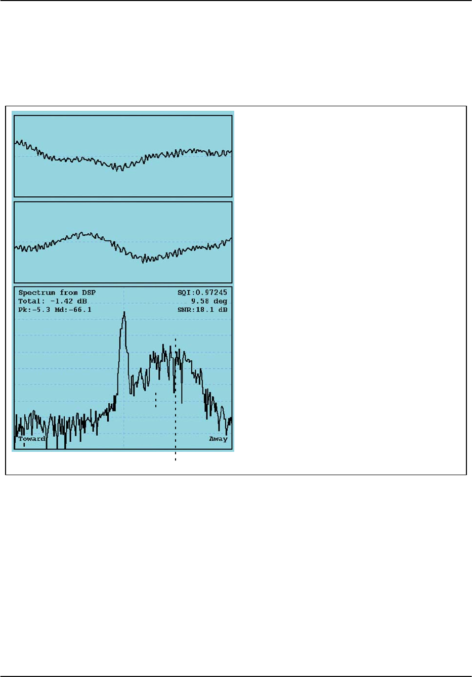
reader is referred to Doviak and Zrnic’s text on the subject. The top part of Figure 5–3 shows I

and Q values for a simulated time series using the ascope utility.

There are two broad categories of time series signal processing:

STime Domain Processing using the I and Q samples directly to calculate

“autocorrelations” and then using the autocorrelations to compute the moments. This is

used by many systems since the algorithms are very efficient requiring minimal storage

and computational power. However, time domain algorithms are generally not adaptive

or very flexible.

SFrequency Domain Processing using the I and Q samples to calculate a Doppler power

spectrum and then applying algorithms, such as clutter filtering or 2nd trip echo

filtering/extraction, in the frequency domain. The Doppler spectrum is then inverted to

obtain the autocorrelation functions and these are used to calculate the moments. The

frequency domain is well suited to more complex adaptive algorithms, i.e., where the

processing algorithm is optimized for the data.

The RVP8 supports the concept of “major modes” or processing modes to process the time

series. Currently the following major modes are supported by SIGMET:

SDFT/FFT Mode is a frequency domain approach which is used for most operational

processing applications. There are a variety of clutter filtering options, including the

GMAP algorithms (Gaussian Model Adaptive Processing).

SPulse Pair Processing or PPP Mode is a time domain approach that is used primarily for

dual polarization applications.

SRandom Phase Mode or RPHASE is a frequency domain approach similar to the

DFT/FFT, except that filtering and extraction of both the first and second trip echoes is

supported.

SBatch Mode during which a small batch of low PRF pulses is transmitted (e.g., for 0.1

degree of scanning) followed by a large batch of higher PRF pulses (e.g., for 0.9 degrees

of scanning) to determine which ranges are likely contaminated by second trip echo. This

Processing Algorithms

RVP8 User’s Manual

March 2006

5–16

was developed to support a US WSR88D legacy requirement. It is not supported in

SIGMET’s IRIS software.

The time and frequency domain approaches are described in the sections below.

Figure 5–3: Example of time series and Doppler power spectrum

White Noise

Ground Clutter

Weather Targets

Velocity

0+VuĆVu

Power

Time series of I and Q and the corre-

sponding Doppler power spectrum ob-

tained from the ascope utility using the

built-in simulator. The Doppler spec-

trum displays the radial velocity on the

X-axis over the unambiguous range or

“Nyquist” interval and the power in dB

relative to saturation on the y-axis.

Note that for illustration, this example

is based on 256 time series points (one

point per pulse) which yields 256 spec-

trum components. This is more than is

usually processed in actual operation.

The spectrum shows the three major

components of the Doppler spectrum:

* White noise.

* Ground clutter at zero radial velocity.

* A spectrum of the weather targets

having a Gaussian shape characterized

by the weather power, mean velocity

and width (standard deviation), i.e., the

spectrum moments.

Mean Velocity

Spectrum

Width

Time

AmplitudeAmplitude

Doppler

Spectrum

σv

Processing Algorithms

RVP8 User’s Manual

March 2006

5–17

5.2.2 Frequency Domain Processing- Doppler Power Spectrum

The Doppler power spectrum, or simply the “Doppler spectrum”, is the easiest way to visualize

the meteorological information content of the time series. The bottom part of Figure 5–3 shows

an example of a Doppler power spectrum for the time series shown in the upper part of the

figure. The figure above shows the various components of the Doppler spectrum, i.e., typically

there is white noise, weather signal and ground clutter. Other types of targets such as sea clutter,

birds, insects, aircraft, surface traffic, second trip echo, etc. may also be present.

The “Doppler power spectrum” is obtained by taking the magnitude squared of the input time

series, i.e. for a continuous time series,

S(w)+|F{s(t)}|2

Here S denotes the power spectrum as a function of frequency ω, and F denotes the Fourier

transform of the continuous complex time series s(t). The Doppler power spectrum is

real-valued since it is the magnitude squared of the complex Fourier transform of s(t).

In practice a pulsed radar operates with discrete rather than continuous time series, i.e., there is

an I and Q value for each range bin for each pulse. In this case we use the discrete Fourier

transform or DFT to calculate the discrete power spectrum. Note that in the special case when

we have 2n input time series samples (e.g., 16, 32, 64, 128, ...), we use the fast Fourier transform

algorithm (FFT), so called because it is significantly faster than the full DFT.

The DFT has the form:

Sk+|DFTk{wmsm}|2+Ťȍ

m+0

wmsme*j(2pńM)mkŤ2

Typically a weighting function or “window” wm is applied to the input time series sm to mitigate

the effect of the DFT assumption of periodic time series. The RVP8 supports different windows

such as the Hamming, Blackman, Von Han, Exact Blackman and of course the rectangular

window for which all spectral components are weighted equally. The typical form of a spectrum

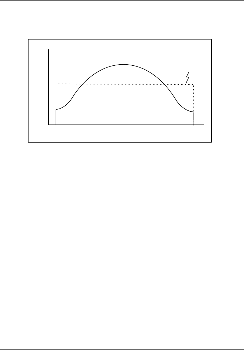
Processing Algorithms

RVP8 User’s Manual

March 2006

5–18

window is shown in the figure below which illustrates how the edge points of the time series are

de–emphasized and the center points are over emphasized. The dashed line would correspond to

the rectangular window. Note that the “gain” of the window is set to preserve the total power.

Time/Sample Index

Weight

Rectangular

Figure 5–4: Typical form of a time series window

Even though the window gain can be adjusted to conserve the total power, there is an effective

reduction in the number of samples which increases the variance (or uncertainty) of the moment

estimates. For example the variance of the total power is greater when computed from a

spectrum with Blackman weighting as compared to using a rectangular window. This is because

there are effectively fewer samples because of the de-emphasis of the end points. This is a

negative side to using a window.

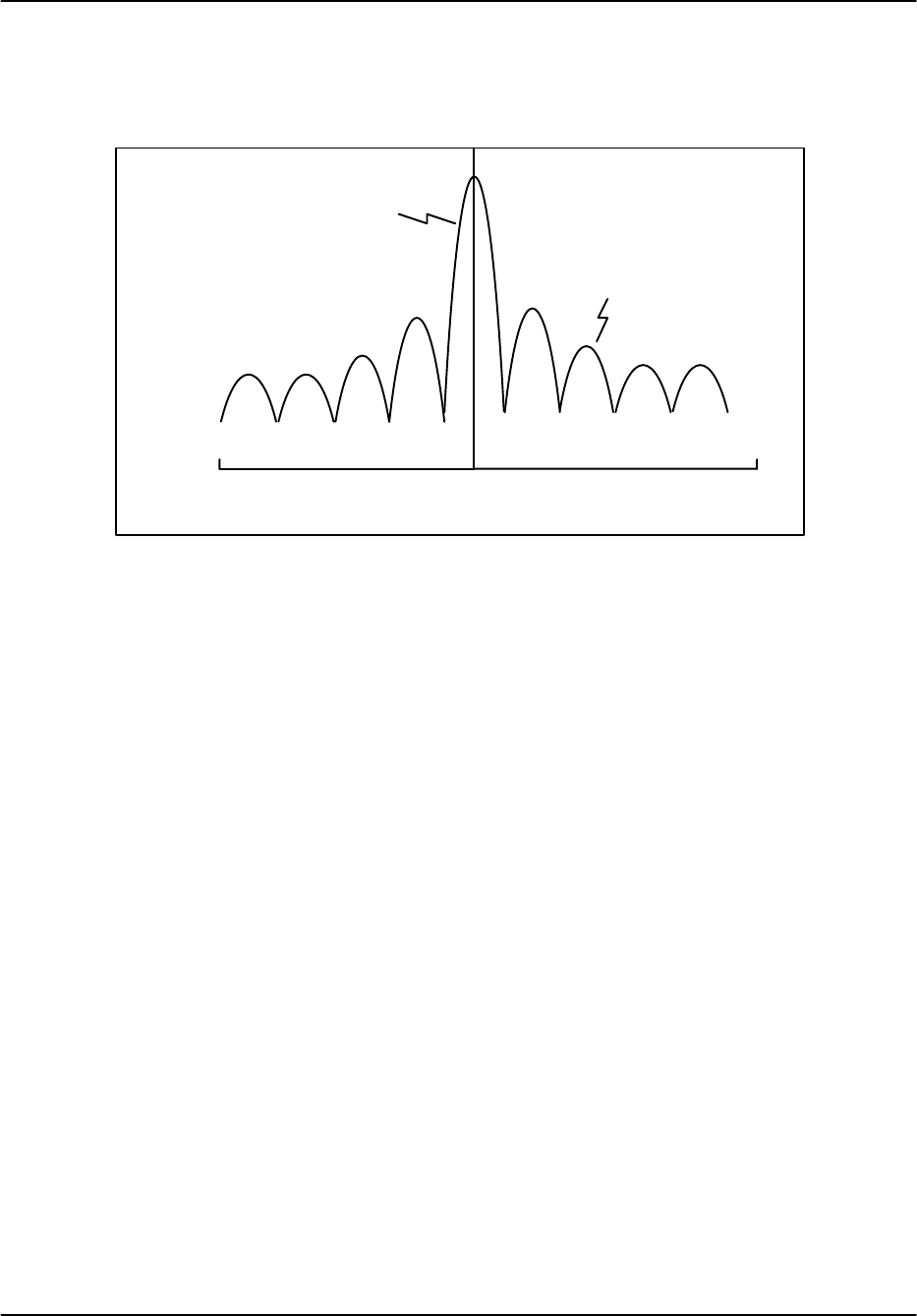
The DFT of the window itself is known as its impulse response which shows all of the

frequencies that are generated by the window itself. A generic example is shown in Figure 5–5

below which illustrates that these “side lobe” frequencies can have substantial power. This is not

a problem for weather signals alone, but if there is strong clutter mixed in, then the side lobe

power from the clutter can obscure the weaker weather signals. The rectangular window has the

worst sidelobes, but the narrowest window width. However, the rectangular window provides the

Processing Algorithms

RVP8 User’s Manual

March 2006

5–19

lowest variance estimates of the moment parameters (in the absence of clutter. More

“aggressive” windows have lower side lobe power at the expense of a broader impulse response

and an increased variance of the moment estimates.

Frequency

Power

M/20

Side Lobes

ĆM/2

Window Width

Figure 5–5: Impulse response of a typical window

So in summary of the DFT approach and spectrum windows:

SWhen the clutter is strong, an aggressive spectrum window is required to contain the

clutter power so that the side lobes of the window do not mask the weather targets. The

side lobe levels of some common windows are:

Rectangular 12 dB

Hamming 40 dB

Blackman 55 dB

SMore aggressive windows typically have a wider impulse response. This effectively

increases the spectrum width. Rectangular is narrow, Hamming intermediate and

Blackman the widest.

SWindows effectively reduce the number of samples resulting in higher variance moment

estimates. Rectangular is the best case, Hamming is intermediate and Blackman provides

the highest variance moment estimates.

These facts suggest the best approach is to use the least aggressive window possible in order to

contain the clutter power that is actually present- i.e., an adaptive approach is the best.

Processing Algorithms

RVP8 User’s Manual

March 2006

5–20

5.2.3 Autocorrelations

The final spectrum moment calculation (for total power or SNR, mean velocity and spectrum

width) in all processing modes is based on autocorrelation moment estimation techniques.

Typically the first three lags are calculated, denoted as R0, R1 and R2. However, there are two

ways to calculate these, i.e., time domain or frequency domain calculation. In the PPP mode for

dual polarization, the autocorrelations are computed directly in the time domain while in the

DFT mode, they are computed by taking the inverse DFT the Doppler power spectrum in the

frequency domain. Note that only the first three terms need be calculated in the inverse DFT

case. The time domain and frequency domain techniques are nearly identical except that the

method of taking the inverse DFT of the power spectrum relies on the assumption that the time

series is periodic. Another difference is that for time domain calculation only a rectangular

weighting is used.

The time domain calculation of the autocorrelations and the corresponding physical models are:

Parameter and Definition Physical Model

To+1

Mȍ

n+1

sn*sngrgt(S)C))N

Ro+1

Mȍ

n+1

sȀ*

nsȀngrgtS)N

R1+1

M*1ȍ

M*1

n+1

sȀ*

nsȀn)1grgtSejpVȀ*p2W2ń2

R2+1

M*2ȍ

M*2

n+1

sȀ*

nsȀn)2grgtSej2pVȀ*2p2W2

where M is the number of pulses in the time average. Here, sȀ denotes the clutter-filtered time

series, s denotes the original unfiltered time series and the * denotes a complex conjugate. gr and

gt represent the transmitter and receiver gains, i.e., their product represents the total system gain.

Since the RVP8 is a linear receiver, there is a single gain number that relates the measured

autocorrelation magnitude to the absolute received power. However, since many of the

algorithms do not require absolute calibration of the power, the gain terms will be ignored in the

discussion of these. To for the unfiltered time series is proportional to the sum of the

meteorological signal S, the clutter power C and the noise power N. R0 is equal to the sum of

the meteorological signal S and noise power N which is measured directly on the RVP8 by

periodic noise sampling. To and R0 are used for calculating the dBZ values- the equivalent radar

reflectivity factor which is a calibrated measurement. The physical models for R0,R1 and R2

correspond to a Gaussian weather signal and white noise as shown in Figure 5–3. W is the

spectrum width and V’ the mean velocity, both for the normalized Nyquist interval on [–1 to 1].

The autocorrelation lags above and the corresponding physical models have five unknowns: N,

S, C, V’, W. Because the R1 and R2 lags are complex, this yields, effectively, five equations in

five unknowns using the constraint provided by the argument of R1. This closed system of

equations can be solved for the unknowns which is the basis for calculating the moments from

the autocorrelations.

Processing Algorithms

RVP8 User’s Manual

March 2006

5–21

5.2.4 Angle Synchronization

The exact value of M that is used for each time average will generally be the “Sample Size” that

is selected by the SOPRM command (See Section 6.3). However, when the RVP8 is in PPP

mode and antenna angle synchronization is enabled, the actual number of pulses used may be

limited by the number that fit within each ray’s angular limits at the current antenna scan rate.

The value of M will never be greater than the SOPRM Sample Size, but it may sometimes be

less. For example, at 1KHz PRF, 20_/sec scan rate, 1_ ray synchronization, and a Sample Size

of 80, there will be 50 pulses used for each ray (not 80). Note, however, that the number of

pulses used in the “batched” (non-PPP) modes will always be exactly equal to the Sample Size,

since those modes are allowed to use overlapping pulses.

5.2.5 Clutter Filtering Approaches

Each major mode implements clutter filtering as follows:

SDFT Mode uses frequency domain clutter filters.

SPPP Mode, used only for dual polarization. No clutter filtering is done in the PPP mode

since this will typically damage the polarization information.

SRandom Phase Mode uses frequency domain clutter filters.

SBatch Mode uses a simple DC removal for the small batch clutter filter. The high PRF

large batch is then processed using the DFT mode.

In previous versions of SIGMET processors, an IIR (infinite implodes response) filter was

offered. The IIR filter, while requiring minimal storage and computation, has three major

drawbacks:

SThe infinite impulse response requires a settling time when a transient occurs such as a

PRF change, or a spike clutter target. During the settling time, the transient response

degrades the performance of the filter.

SThe filter is fixed width in the Nyquist interval. This means that it may be sufficiently

wide to remove moderate or weak clutter, but may not be wide enough to remove all of

the clutter when the clutter power is very strong and consequently wider in the Nyquist

interval. This causes operators to select wider filters than necessary so that strongest

clutter is adequately removed.

SThe filter does significant damage to overlapped (zero velocity) weather signals, i.e.,

these will be significantly attenuated by the filter.

With the advent of the high speed processors such as the RVP8, there is sufficient storage and

computational power to implement frequency domain filters that, in some cases, are adaptive.

Because of the superiority of these filters, the legacy time domain IIR approach is no longer used

in the RVP8. The only mode that uses time domain filtering is the Batch mode for the low PRF

pulses (subtraction of the average I and Q to remove the DC component).

The various frequency domain filters available in the RVP8 are configured using the “mf” setup

command (Section 3.2.3). These are:

Processing Algorithms

RVP8 User’s Manual

March 2006

5–22

SType 0: Fixed width filters with interpolation

SType 1:Variable width single slope adaptive processing

SType 2: Gaussian model adaptive processing (GMAP)

These filters are described in in the sections detail below.

Processing Algorithms

RVP8 User’s Manual

March 2006

5–23

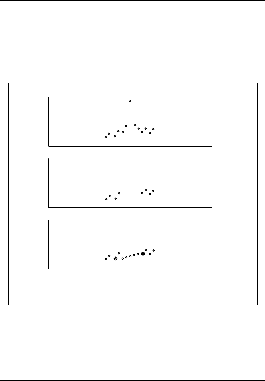
5.2.5.1 Fixed Width Clutter Filters

This filter, illustrated in Figure 5–6, removes a specified number of spectrum components

(5 in the example) and then interpolates across the gap using the minimum of a specified

number of “edge points” (2 in the example) to anchor the interpolation at each end of the gap.

This is a fairly simple legacy approach that uses interpolation to repair the damage caused

by the removal of components.

Figure 5–6: Example of fixed width

Spectrum with ground clutter

-20

-40

-60

dB Power

Velocity

0+Vu-Vu

Remove 5 interior points

-20

-40

-60

dB Power

Find minimum of 2 edge points

Interpolate across 5 center points

-20

-40

-60

dB Power

This procedure attempts to preserve the noise level and/or overlapped weather targets. The result

is that more accurate estimates of dBZ are obtained. In extreme cases when the weather

spectrum is very narrow, there can still be some attenuation of weather of a broad filter is

selected.

Processing Algorithms

RVP8 User’s Manual

March 2006

5–24

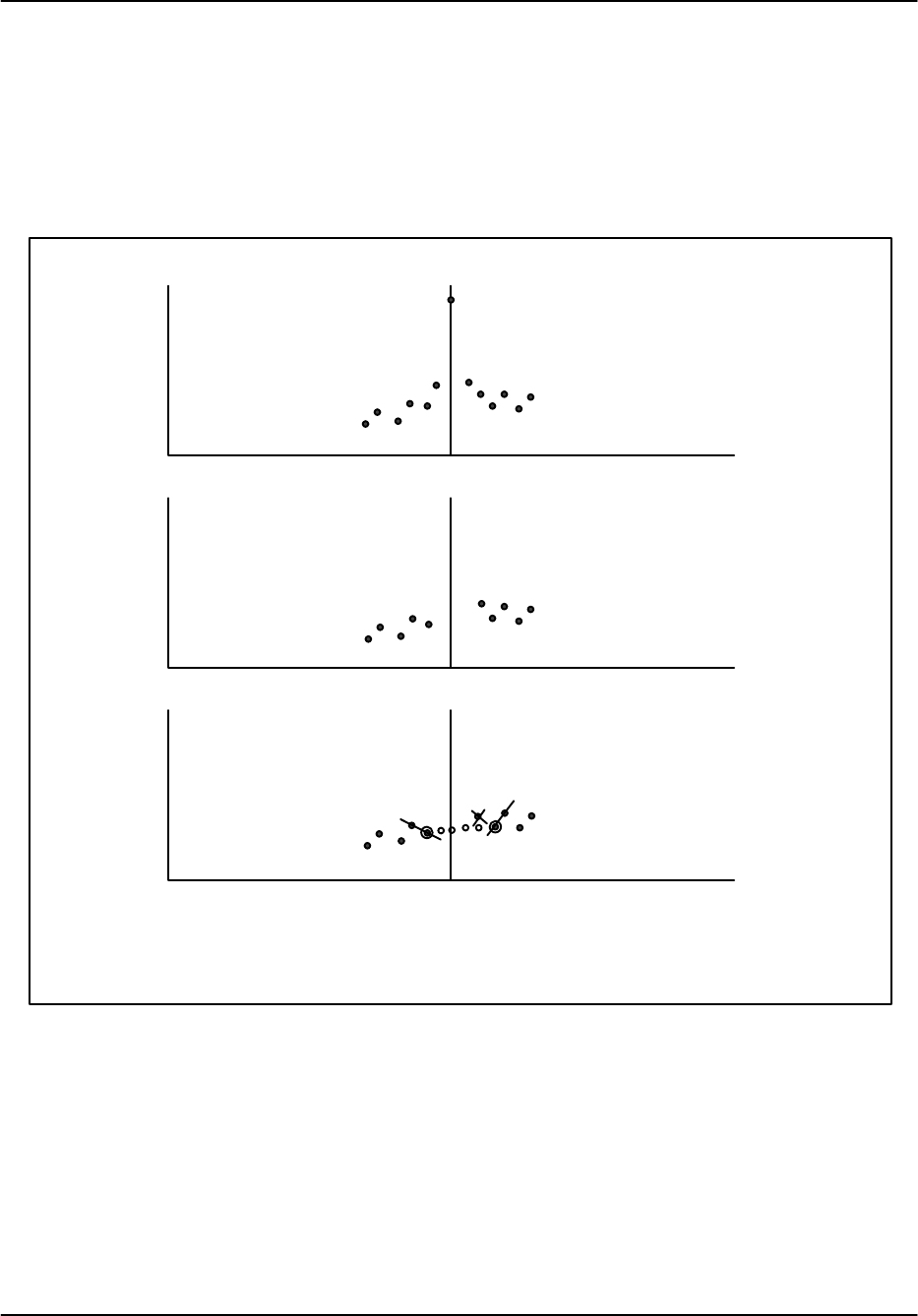
5.2.5.2 Variable Width Clutter Filter

This is similar in many ways to the fixed width filter except that the algorithm attempts to

extend the boundary of the clutter by determining which is the first component outside the

clutter region to increase in power. The filter is illustrated in the figure below.

Figure 5–7: Variable Width Clutter Filter

Spectrum with ground clutter

-20

-40

-60

dB Power

Velocity

0+Vu-Vu

Remove 3 interior points

-20

-40

-60

dB Power

Use slope to extend the clutter boundĆ

ary. Then find the minimum of the 2

edge points and interpolate.

-20

-40

-60

dB Power

In the example above, the minimum number of points to reject is set to 3. The filter starts

at zero velocity and checks the slope to determine the point at which the power starts to in-

crease. In the example, this results in the filter being extended by one point on the right. Note

that there is a selectable maximum number of points that the filter will “hunt”. The use of

the edge points for interpolation is identical to the fixed width case.

This filter allows users to specify a narrower nominal filter than the fixed width case and then

when the clutter is strong, this width is extended by the algorithm (the “hunt”). The interpola-

tion attempts to preserve any overlapped clutter and weather.

Processing Algorithms

RVP8 User’s Manual

March 2006

5–25

5.2.5.3 Gaussian Model Adaptive Processing (GMAP)

GMAP is a new adaptive technique developed at SIGMET that is possible on a high-speed

processor such as the RVP8. GMAP has the following advantages as compared to fixed width

frequency domain filters or time domain filtering such as the IIR approach:

SThe width adapts in the frequency domain to adjust for the effects of PRF, number of

samples and the absolute amplitude of the clutter power. This means that minimal

operator intervention is required to set the filter.

SIf there is no clutter present, then GMAP does little or no filtering.

SGMAP repairs the damage to overlapped (near zero velocity) weather targets.

SThe DFT window is determined automatically to be the least aggressive possible to

remove the clutter. This reduces the variance of the moment estimates.

The GMAP algorithm is described below.

GMAP Model Assumptions

GMAP makes several assumptions about the model for clutter, weather and noise, i.e.,

SThe spectrum width of the weather signal is greater than that of the clutter. This is a

fundamental assumption required of all Doppler clutter filters.

SThe Doppler spectrum consists of ground clutter, a single weather target and noise.

Bi-modal weather targets, aircraft or birds mixed with weather would violate this

assumption.

SThe width of the clutter is approximately known. This is determined primarily by the

scan speed and to a lesser extent by the climatology of the local clutter targets. The

assumed width is used to determine how many interior clutter points are removed.

SThe shape of the clutter is approximately Gaussian. This shape is used to calculate how

many interior clutter points are removed.

SThe shape of the weather is approximately Gaussian. This shape is used to reconstruct

filtered points in overlapped weather.

GMAP Algorithm Steps

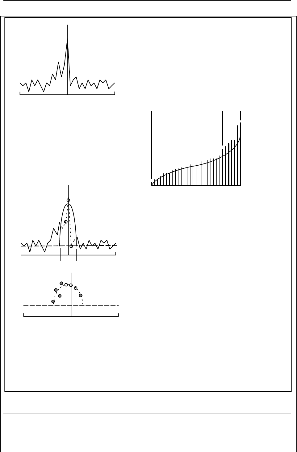
The steps used to implement the GMAP approach are shown schematically in Figure 5–8

and summarized below.

SStep 1: Window and DFT

First a Hamming window weighting function is applied to the IQ values and a discrete

Fourier transform (DFT) is then performed. This provides better spectrum resolution than

a fast Fourier Transform (FFT) which requires that the number of IQ values be a power

of 2. Note that if the requested number of samples is exactly a power of 2, then an FFT

is used.

Processing Algorithms

RVP8 User’s Manual

March 2006

5–26

Step 1: Window and DFT

Apply window and DFT the input time series to obtain the Doppler

power spectrum. A Hamming window is used for the first trial.

Step 3: Remove clutter points

Use the total power of the three central spectrum points (indicated by the

three open circles) to fit a Gaussian having the selected nominal spec-

trum width in m/s (a function of the number of spectrum samples, PRF

and wavelength). The points within the intersection of the Gaussian clut-

ter and the noise level (the “Clutter Region”) are discarded (indicated by

the dashed lines).

Percentage of spectrum points having power < I

0 100%

dB Power, I

Noise Region

Signal/Clutter

Region

Vu–Vu

Power dB

0Vu–Vu

Power dB

0Vu–Vu

Power

Clutter

Region Step 4: Replace clutter points

Dynamic Noise Case: Using the components which have been deter-

mined to be neither clutter nor noise (indicated by the filled circles), fit

a Gaussian and fill-in the clutter points that were removed in the previous

step (indicated by the open circles). Then re-fit the Gaussian with the re-

placement values inserted. Repeat the iteration until the computed power

does not change by more than 0.2dB AND the velocity does not change

by more than 0.5% of the Nyquist velocity.

Fixed Noise Case: Similar except the spectrum points that are larger than

the noise level are used.

Step 2 (Optional): Dynamic noise power

If the noise level is not known, or if GMAP is recalculated using the

Blackman window for CSR>40 dB, then this step is performed. Re-or-

ganize the spectrum components in ascending order of intensity. The

theoretical relationship for noise is the curved line. The sum of the

power in the range 5% to 40% is calculated. This is used to determine

the noise level by comparing with the sum value corresponding to the

theoretical curve. Next, the power is summed beyond the 40% point

for both the actual and theoretical rank spectra. The point where the ac-

tual power sum exceeds the theoretical value by 2 dB determines the

boundary between the noise region and the signal/clutter region.

Noise

Level

Noise

Level

Step 5: Recompute GMAP with optimal window

Determine if the optimal window was used based on the clutter-to-signal ratio (CSR)

IF CSR > 40 dB repeat GMAP using a Blackman window and dynamic noise calculation.

IF CSR > 20 dB repeat GMAP using a Blackman window. Then if CSR>25dB use Blackman results.

IF CSR < 2.5 dB repeat GMAP using a rectangular window. Then if CSR < 1 dB use rectangular re-

sults.

ELSE accept the Hamming window result.

Figure 5–8: GMAP Algorithm Steps

Processing Algorithms

RVP8 User’s Manual

March 2006

5–27

SAs mentioned in Section 5.2.2, when there is no or very little clutter, use of a rectangular

weighting function leads to the lowest-variance estimates of intensity, mean velocity and

spectrum width. When there is a very large amount of clutter, then the aggressive

Blackman window is required to reduce the “spill-over” of power from the clutter target

into the sidelobes of the impulse response function. The Hamming window is used as the

first guess. After the first pass GMAP analysis is complete, a decision is made to either

accept the Hamming results, or recalculate for either rectangular or Blackman depending

on the clutter-to-signal ratio (CSR) computed from the Hamming analysis. The

recalculated results are then checked to determine whether to use these or the original

Hamming result (see Figure 5–8 for details).

SStep 2: Determine the noise power

In general, the spectrum noise power is known from periodic noise power measurements.

Since the receiver is linear and requires no STC or AGC, the noise power is

well–behaved at all ranges. The only time that the spectrum noise power will differ from

the measured noise power is for very strong clutter targets. In this case, the clutter

contributes power to all frequencies, essentially increasing the spectrum noise level. This

occurs for two reasons: 1) In the presence of very strong clutter, even a small amount of

phase noise causes the spectrum noise level to increase, and 2) There is significant power

that occurs in the window side-lobes. For a Hamming window, the window side lobes are

down by 40 dB from the peak at zero velocity. Thus 50 dB clutter targets will have

spectrum noise that is dominated by the window sidelobes in the Hamming case. The

more aggressive Blackman window has approximately 55 dB window sidelobes at the

expense of having a wider impulse response and larger negative effect on the variance of

the estimates.

SWhen the noise power is not known, it is optionally computed using a dynamic approach

similar to that of Hildebrand and Sekhon (1974). The Doppler spectrum components are

first sorted in order of their power. As shown in Figure 5–8, the sorting places the

weakest component on the left and the strongest component on the right. The vertical

axis is the power of the component. The horizontal axis is the percentage of components

that have power less than the y-axis power value. Plotted on a dB scale, Poisson

distributed noise has a distinct shape, as shown by the curved line in Figure 5–8. This

shape shows a strong singularity at the left associated with taking the log of numbers near

zero, and a strong maximum at the right where there is always a finite probability that a

few components will have extremely large values.

SThere are generally two regions: a noise region on the left (weaker power) and a

signal/clutter region on the right (stronger power). The noise level and the transition

between these two regions is determined by first summing the power in the range 5% to

40%. This sum is used to determine the noise level by comparing with the sum value

corresponding to the theoretical curve. Next, the power is summed beyond the 40% point

for both the actual and theoretical rank spectra. The point where the actual power sum

exceeds the theoretical value by 2 dB determines the boundary between the noise region

and the signal/clutter region.

Processing Algorithms

RVP8 User’s Manual

March 2006

5–28

SFinally there are two outputs from this step: a spectrum noise level and a list of

components that are either signal or clutter

SStep 3: Remove the clutter points

The inputs for this step are the Doppler power spectrum, the assumed clutter width in m/s

and the noise level, either known from noise measurement or optionally calculated from

the previous step. First the power in the three central spectrum components is summed

(DC ±1 component) and compared to the power that would be in the three central

components of a normalized Gaussian spectrum having the specified clutter width and

discretized in the identical manner. This serves as a basis for normalizing the power in

the Gaussian to the observed power. The Gaussian is extended down to the noise level

and all spectral components that fall within the Gaussian curve are removed. The power

in the components that are removed is the “clutter power”.

SA subtle point is the use of the three central points to do the power normalization of the

actual vs the idealized spectrum of clutter. This is more robust than using a single point

since for some realizations of clutter targets viewed with a scanning antenna, the DC

component is not necessarily the maximum. Averaging over the three central components

is a more robust way to characterize the clutter power.

SThe very substantial algorithmic work that has been done thus far is to eliminate the

proper number of central points. The operator only has to specify a nominal clutter width

in m/s. This means that the operator does not need to consider the PRF, wavelength or

number of spectrum points- GMAP accounts for these automatically.

SA key point is that in the event that the sum of the three central components is less than

the corresponding noise power, then it is assumed that there is no clutter and all of the

moments are then calculated using a rectangular window. If the power in the three

central components is only slightly larger than the noise level, then the computed width

for clutter removal will be so narrow that only the central (DC) point shall be removed.

This is very important since, if there is no clutter then we want to do nothing or at worst

only remove the central component.

SBecause of this behaviour, there is no need to do a clutter bypass map, i.e., turn-off the

clutter filter at specific ranges, azimuths and elevation for which the map declares that

there is no clutter. Because of the day-to-day variations in the clutter and the presence of

AP, the clutter map will often be incorrect. Since GMAP determines the no-filter case

automatically and then processes accordingly, a clutter map is not required.

SStep 4: Replace clutter points

The assumption of a Gaussian weather spectrum now comes into play to replace the

points that have been removed by the clutter filter. There are two cases depending on

how the noise level is determined under Step 2, i.e., the dynamic noise case and the fixed

noise level case.

SDynamic noise level case: From Step 2, we know which spectrum components are

noise. From Step 3 we know which spectrum components are clutter. Presumably,

everything that is left is weather signal. An inverse DFT using only these components is

Processing Algorithms

RVP8 User’s Manual

March 2006

5–29

performed to obtain the autocorrelation at lags 0, 1. This is very computationally efficient

since there are typically few remaining points and only the first two lags need be

calculated. The pulse pair mean velocity and spectrum width are calculated using the

Gaussian model (e.g., see Doviak and Zrnic, 1993). Note that since the noise has already

been removed, there is no need to do a noise correction. The Gaussian model is then

applied using the calculated moments to determine a substitution value for each of the

spectrum components that were removed in Step 3.

SIn the case of overlapped weather as shown in the Figure 5–8 example, the replacement

power is typically too small. For this reason, the algorithm recomputes R0 and R1 using

both the observed and the replacement points and computes new replacement points. This

procedure is done iteratively until the power difference between two successive iterations

is less than 0.2 dB and the velocity difference is less than 0.5% of the Nyquist interval.

SIn summary of this step, the Gaussian weather model is used to repair the filter bias, i.e.,

the damage that is caused by removing the clutter points. An IIR filtering approach

makes no attempt to repair filter bias, rather the filter simply “digs a hole” into

overlapped weather.

SStep 5: Check for appropriate window and recalculate the moments if necessary.

The clutter power is known from the spectrum components that were removed in Step 3.

Since the weather spectrum moments and the noise are also known from Step 4, the CSR

can be calculated. The value of the CSR, is used to decide whether the Hamming

window is the most appropriate. The scenarios are described in Figure 5–8. The end

result is that very weak clutter is processed using a rectangular window, moderate clutter

a Hamming window, while severe clutter requires a Blackman window. Note that if no

clutter were removed in Step 3, then the spectrum is processed with a rectangular

window.

SThe benefit of adaptive windowing is that the least aggressive window is used for the

calculation of the spectrum moments, resulting in the minimum variance of the moment

estimates.

GMAP Configuration

The ’mf’ command in the dspx TTY setups is used to configure GMAP filters. In the section

for the spectrum filters select filter “Type 2” and specify the width of the ground clutter in

m/s. This width is determined largely by your antenna rotation rate so you will want to con-

figure several widths to deal with the different rotation rates in your operational scenario.

An example might be filters indexed 1-5 corresponding to widths from 0.1 to 0.5.

A good practice is to make a scan on a clear day while using ascope or other utility and ob-

serve what the actual width of the clutter is for your various scan rates. You will need to turn-

off the clutter filtering to do this (pick “filter 0” for the all pass filter).

Example of Implementation

GMAP has undergone extensive evaluation for use in the US WSR88D ORDA network up-

grade (Ice et al, 2004). They conclude that GMAP meets the ORDA requirements. Their

Processing Algorithms

RVP8 User’s Manual

March 2006

5–30

study was based on a built-in simulator that is provided as part of the RVP8 and the ascope

utility. The simulator allows users to construct Doppler spectra, process them and evaluate

the results (Sirmans and Bumgarner, 1975). This is an essential tool for evaluating the system

performance.

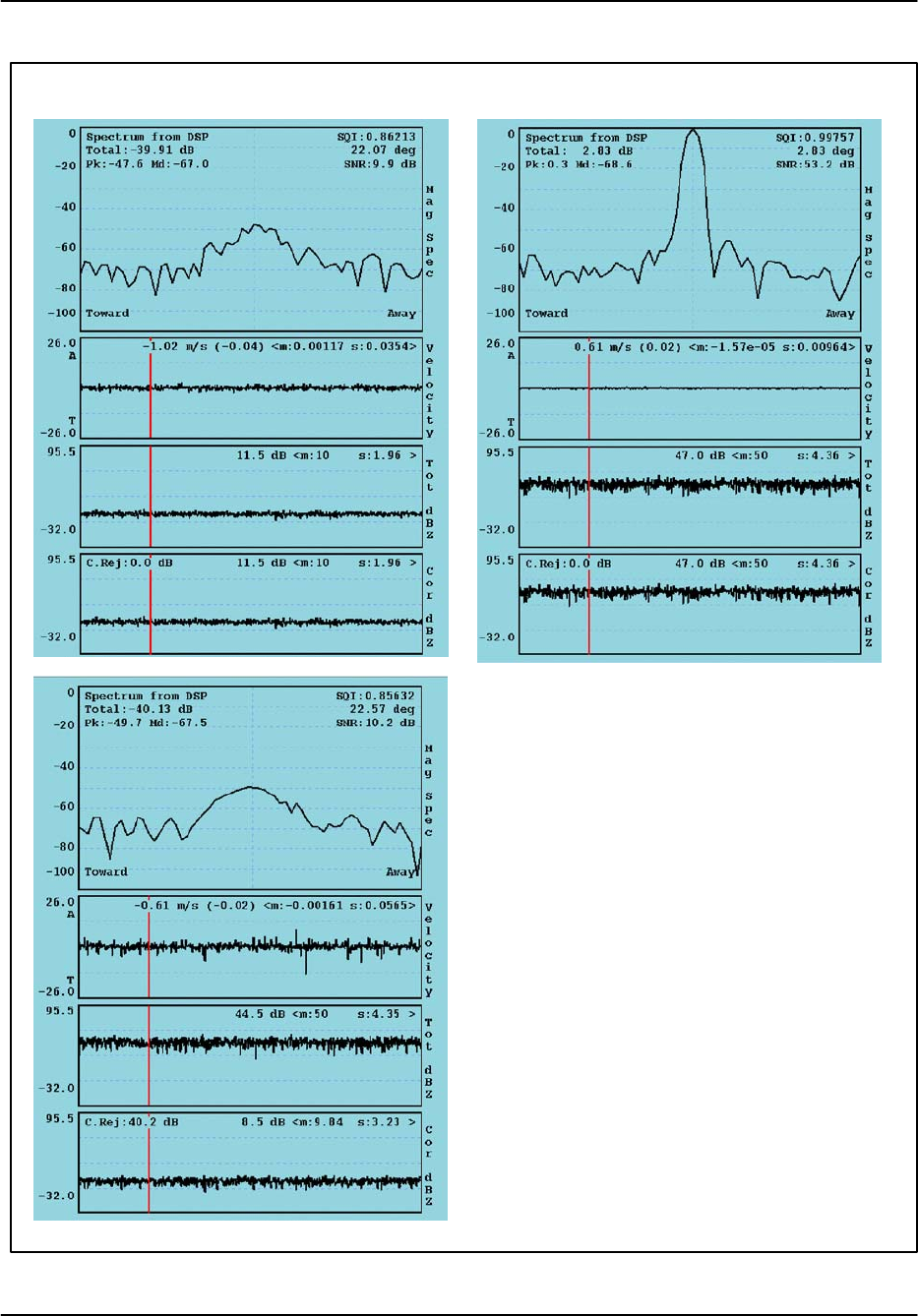
Figure 5–9 shows an example of the simulations for the very difficult case when the weather

has zero velocity, i.e., it is perfectly overlapped with clutter. The upper left graph shows the

weather signal with –40 dB power without any clutter and without any GMAP filtering. The

graph at the upper right shows the same spectrum with 0 dB of clutter power added for a clut-

ter width of 0.012 (0.3 m/s at S band, 1000 Hz PRF). This is a CSR of 40 dB. The panel at

the lower left shows the weather signal after GMAP filtering.

In each of the moment plots, there are several values that are displayed. The left-most num-

ber shows the value at the range cursor which is positioned as indicated by the vertical line.

To the right, the “m” value is the mean and the “s” value the standard deviation as averaged

over all range bins (1000 in this example). For velocity these are in normalized units ex-

pressed as a fraction of the Nyquist interval. For reflectivity the values are in dB.

Some key points are:

SThe mean velocity is correctly recovered as expected (the “m” value in the plot), but the

standard deviation is higher (0.06 vs 0.04 in normalized units).

SThe “Cor dBZ” shows 40.2 dB of “C.Rej”. This is the difference between the “Tot dBZ”

and the “Cor dBZ” values. The expected value is 40 dB in this case. This indicates that

GMAP has recovered the weather signal in spite of the aggressive clutter filtering that is

required.

SThe standard deviation of the “Tot dBZ” is greater in the weather plus clutter (4.35

normalized units) as compared to the weather-only case. This is caused by the

fluctuations in the clutter power in the Gaussian clutter model.

SThe standard deviation of the Cor dBZ after GMAP filtering, while not as low as for the

weather-only case are lower than the weather plus clutter case. In other words, the

GMAP processing removes some of the high variance in the dBZ estimates that is caused

by clutter, but is not quite as good as doing nothing.

Processing Algorithms

RVP8 User’s Manual

March 2006

5–31

Weather only Weather plus clutter

Simulation Characteristics

Clutter Weather Units

Power 0 –40 dB

Vel 0 0 Any

Width 0.012 0.1 Normalized

PRF 1000 Hz Window Blackman

ModeFFT Samples 64

“Mag Spec”: Doppler Spectrum in dB Units spanning

the Nyquist interval.

“Velocity”: Mean velocity of the spectrum in over Ny-

quist interval. Mean “m” and standard deviation values

“s” are for the normalized interval ±1.

“Tot dBZ”: Power in dB of weather and clutter. Mean

“m” and standard deviation values “s” are in dB.

“Cor dBZ”: Power in dB after GMAP filtering. Mean

“m” and standard deviation values “s” are in dB.

“<m: ...s: ...>” mean and standard deviation over all

ranges, in this case 1000 range bins.

Figure 5–9: GMAP example

Processing Algorithms

RVP8 User’s Manual

March 2006

5–32

5.2.6 Range averaging and Clutter Microsuppression

The next step (optional) is to perform range averaging. Range averaging can be performed over

2, 3, ..., 16 bins. This is accomplished by simply averaging the T0,R0,R1 and R2 values. This

reduces the number of bins in the final output to save processing both in the RVP8 and in the

host computer.

At the user’s option, the range averaged data can be restricted to include only those bins which

have an estimated clutter-to-signal ratio that falls within the CCOR threshold interval. By

excluding isolated point clutter targets from the range average the sub-clutter visibility of the

averaged data is increased. Specifically, the Doppler test that is applied to each bin in order that

it contribute to the overall sum is:

10 log R0*10 log T0uCCORthresh .

5.2.7 Reflectivity

The corrected reflectivity Z is output using a log scale based on the following equation:

dBZ +10 logƪT0*N

Nƫ)dBZo)20 log r)ar )CCOR

This equation is simply a dB version of the familiar radar equation for distributed targets. The

relationship between the measured autocorrelation function, the received signal and the noise can

be expressed as:

To+gtgrS)N

where gt and gr represent the transmitter and receiver gains, S is the average back scattered

power from the targets and N is the measured average noise power. Neglecting attenuation and

the contribution of ground clutter (for the moment), the radar equation can be written as.

Z+CSr2+ƪCr2

grgtƫƪr2

oƫƪTo*N

Nƫ

where C is the radar constant and ro is a reference range which we will later set to 1 km. This is

identical to the first three terms of the dB version of the equation with the definition that:

Zo+Cr2

grgt+Cr2

oIowhere Io+N

grgt

Zo is called the calibration reflectivity factor. It is the equivalent radar reflectivity factor at the

reference range when the return signal power is equal to the noise power (SNR=0 dB). It is

sometimes called the minimum detectable dBZ at 1 km, though it is more correct to call it the

0dB SNR detection level (See Figure 5–10). The parameter Io is the measured noise power at IF

with appropriate calibration for the system gain. Calibration of the RVP8 involves defining the

radar constant C and measuring the value of Io. This is discussed in detail in Section 5.4.

Processing Algorithms

RVP8 User’s Manual

March 2006

5–33

Essentially, the measurement of Io is based on the measurement of the system noise at the time

of calibration. However, if the receiver gain were to change after calibration, the use of periodic

noise sampling properly corrects for this. For example, if the receiver gain were to change by a

factor k, then we would measure a noise value of kN and an autocorrelation value of kTo, i.e.,

Z+CSr2+ƪCr2

grgtƫƪr2

oƫƪ

o*kN

kN ƫ

Thus the k’s cancel to give us the same result for Z. This makes the approach robust to system

gain fluctuations. Another way of saying this is that as long as the system sensitivity (noise

figure) does not change, then the system does not require re-calibration.

The individual terms in the dB form of the equation are summarized below.

1st Term : 10 logƪT0*N

Nƫ: Signal to Noise Ratio

The effect of this term is to subtract the measured noise and then divide by that noise. The

result is a Signal-to-Noise ratio.

2rd Term: dBZo : Calibration Reflectivity (see discussion above)

dBZo is the minimum detectable dBZ at a reference range ro=1 km,

3th Term: 20 log r : Range Normalization

This term is the ƪr

roƫ2 range normalization expressed in dB form.

4th Term: ar : Gaseous Attenuation Correction

This term accounts for gaseous attenuation. The constant a is set in the RVP8 EEROM since

it is a function of wavelength. For a C-band system the default value is 0.016 dB per km (for

two-way path attenuation).

5th Term: CCOR: Clutter Correction

This term corrects for the measured ground clutter. It’s derivation is discussed in section

5.2.11.

Processing Algorithms

RVP8 User’s Manual

March 2006

5–34

5.2.8 Velocity

For a Doppler power spectrum that is symmetric about its mean velocity, the velocity is obtained

directly from the argument of the autocorrelation at the first lag, i.e.,

V+l

4ptsq1 where q1+arg ǊR1ǋ.

l is the radar wavelength, ts is the sampling time (1/PRF). q1 is constrained to be on the

interval [*p,p]. When q1+" p , then V+" Vu where the unambiguous velocity is ,

Vu+l

4ts .

If the absolute value of the true velocity of the scatterers is greater than Vu , then the velocity

calculated by the RVP8 is folded into the interval ƪ*Vu,Vuƫ , which is called the Nyquist

interval. Folding is usually easily recognized on a color display by a discontinuous jump in

velocities. For example, if the true velocity is Vu)DV, then the velocity calculated by the

RVP8 is *Vu)DV, which is 2Vu away from the true mean velocity.

For 8-bit outputs, rather than calculating the absolute velocity in scientific units, the RVP8

calculates the mean velocity for the normalized Nyquist interval [–1,1], i.e., the output values

are,

VȀ+q1

For example, an output value of –0.5 corresponds to a mean velocity of *Vuń2. The

normalized velocity VȀ is more efficient use of the limited number of bits.

5.2.9 Spectrum Width Algorithms

The spectrum width is a measure of the combined effects of shear and turbulence. To a lesser

extent, the antenna rotation rate can also effect the spectrum width. At high elevation angles, the

fall speed dispersion of the scatterers also effects spectrum width.

There are two choices for the spectrum width algorithm used in the RVP8, depending on the

speed and accuracy that are required for the application:

R0,R1 “fast” algorithm valid when SNR >> 10 dB

R0,R1,R2 “accurate” algorithm for SNR >> 0 to 5 dB

The approach used is selected in the SOPRM command. The two approaches are described below:

R0,R1Width Algorithm

Given samples of the Doppler autocorrelation function, numerous estimates of spectral vari-

ance can be computed (Passarelli & Siggia, 1983). The particular estimator used by the

RVP8 employs the magnitudes of R0 and R1 and assumes that the Doppler spectrum is

Gaussian (usually an acceptable assumption) and that the signal-to-noise ratio is large. Spe-

cifically we have (similar to Srivastava, et al 1979):

Variance +2ln

ƪRo

|R1|ƫ+*2ln

[SQI]

Processing Algorithms

RVP8 User’s Manual

March 2006

5–35

where “ln” represents the natural logarithm. This can be compared to the expression in the

preceding section for SQI to illustrate that this expression for the variance is only valid when:

SNR

SNR )1[1

which occurs when the SNR is large.

This variance estimator is normalized to the Nyquist interval in units of [*p,p]. Thus, for

example, a variance of p2ń25 would be obtained from a Gaussian spectrum having a stan-

dard deviation equal to one fifth of the total width of the plotted spectral distribution. For

scientific purposes, the spectrum width (standard deviation) is more physically meaningful

than the variance, since it scales linearly with the severity of wind shear and turbulence. For

these reasons, the width W is output by the RVP8:

W+Variance

Again, for efficient packing in 8-bits, width is normalized to the Nyquist interval [–1, 1 ].

For the example given above, the output width W would be (1/5). To obtain the width in me-

ters per second, one multiplies the output width by Vu .

R0,R1,R2 Width Algorithm

The width algorithm in this case is similar except that the addition of R2 extends the validity

of the width estimates to weak signals. In this case the variance is:

Variance +2

3lnƪ|R1|

|R2|ƫ

The output width W is then defined as in the previous section.

5.2.10 Signal Quality Index (SQI threshold)

An important feature of the RVP8 is its ability to eliminate signals which are either too weak to

be useful, or which have widths too large to justify further analysis. This is done via the signal

quality index (SQI) which is defined as:

SQI +|R1|

The SQI is the normalized magnitude of the autocorrelation at lag 1 and varies between 0 for an

uncorrelated signal (white noise) to 1 for a noise-free zero-width signal (pure tone). Mean

velocity estimates are degraded when the spectrum, width is large or when the signal-to-noise

ratio is weak. The SQI is a good measure of the uncertainty in the velocity estimates and is a

convenient screening parameter to compute. In terms of the Gaussian model, the SQI is :

SQI +SNR

SNR )1e*p2W2

where the SNR is the signal-to-noise ratio. For very large SNR’s the SQI is a function of the

spectrum width only. For a zero-width pure tone (W=0), the SQI is a function of the SNR only

(e.g., for W=0, an SNR of 1 corresponds to SQI=0.5). The SQI threshold is typically set to a

value of 0.4 to 0.5.

Processing Algorithms

RVP8 User’s Manual

March 2006

5–36

5.2.11 Clutter Correction (CCOR threshold)

In addition to calculating the R0,R1 and optional R2 autocorrelation terms, which are based on

filtered time series data, the RVP8 also computes T0 which is the total unfiltered power. By

comparing the total filtered and unfiltered powers at each range bin, a clutter power, and hence a

clutter correction, for that bin can be derived. The clutter correction is defined as,

CCOR +10 log S

C)S+10 log 1

CSR )1

where S is the weather signal power, C is the clutter power and CSR is the clutter-to-signal

ratio. The algorithm for calculating CCOR depends on whether the optional R2 autocorrelation

lag is computed as described below.

R0,R1 Clutter Correction

In this case CCOR is estimated from,

CCORest +10 logƪR0

T0ƫ

+10 logƪS)N

C)S)Nƫ+10 logƪ1)1

SNR

CSR )1)1

SNRƫ

Here, the expression is strictly valid only when the signal-to-noise ratio (SNR=S/N) is large.

Thus when the 2-lag approach is used, the clutter corrections are not as accurate for weak

weather signals. However, the error is typically less than 3 dB.

R0,R1,R2 Clutter Correction

In this case there is enough information to compute the clutter signal and noise power inde-

pendently. The algorithm for CCOR is:

CCORest +10 log S

C)S+10 log 1

CSR )1

The clutter power is computed from:

C+To*Ro+ƪC)S)Nƫ*ƪS)Nƫ

The signal power S is then computed from:

S+|R1| exp p2W2

W is the width that has been previously calculated. This approach yields more accurate re-

sults for the clutter correction in the case of a low SNR.

Processing Algorithms

RVP8 User’s Manual

March 2006

5–37

5.2.12 Weather Signal Power (SIG threshold)

A parameter called SIG is also calculated to provide an estimate of the weather signal-to-noise

ratio in dB for thresholding. The SIG calculation is different depending on the whether the

optional R2 autocorrelation is computed.

R0,R1 Calculation

In this case the SIG is computed as follows:

SIG +10 log ƪT0*N

Nƫ)CCOR

This term represents the SNR after the removal of clutter. The CCOR value is the one de-

scribed for R0,R1 in the previous section.

R0,R1,R2 Calculation

In this case the SIG is computed based on the SNR which is:

SIG +10 log ƪ2pS

R0*2pSƫ

where the signal power S is determined as described in the preceding section.

5.2.13 (Signal+Noise)/Noise Ratio (LOG threshold)

A threshold parameter called LOG is also calculated to provide a signal strength estimate that is

useful for qualifying reflectivity. For historical reasons, the LOG threshold is not the true SNR

(whose dB representation can be both positive and negative) but rather, the ratio of Signal plus

Noise to Noise, which always has a positive representation in dB. Specifically:

LOG +10 logƪT0

Nƫ(when applied to the dBT parameter)

LOG +10 logƪR0

Nƫ(when applied to all other parameters)

Processing Algorithms

RVP8 User’s Manual

March 2006

5–38

5.3 Thresholding

An important feature of the RVP8 is its ability to accept or reject incoming data based on derived

properties of the signals themselves. Typically, “rejected” data are not displayed by the user’s

software, thus making for very clean weather presentations.

5.3.1 Threshold Qualifiers

For data quality control, each RVP8 output parameter can be qualified, i.e., either accepted or

rejected for output, based on four threshold criteria:

ID Criterion Name Pass Criterion

LOG (Signal+Noise)-to-Noise Ratio LOG > threshold

SQI Signal Quality Index SQI > threshold

CCOR Clutter Correction CCOR > threshold

SIG Weather Signal Power SIG > threshold

The calculation of the measured levels (e.g., SQI) for each of these qualifications has been

described in previous sections of this chapter. All four qualification criteria can be switched on

and off independently, and the threshold levels (e.g., SQIthresh ) can each be set independently.

Further, each qualifier test can be AND’d and OR’d with any other. This allows very complex

thresholds criteria to be constructed as required. The four threshold qualifiers are summarized

below.

LOG This is a measure of signal strength that is usually used for the thresholding of

reflectivity data. The default LOG threshold value is 0.5 dB.

SQI The SQI threshold is typically used for velocity and width thresholding since it is a

measure of the coherency. It is a number between 0 and 1 (dimensionless) where 0 is

perfect white noise and 1 is a pure tone (perfect Doppler signal). The default SQI

threshold value is 0.5.

CCOR The clutter correction threshold is typically used to reject measurements when the

clutter in a range bin is very strong (i.e., when the calculated CCOR is a large

negative number in dB). The appropriate value depends on the coherency of the radar

system. The default threshold is set to –25 dB. Threshold values less than this (more

negative) reject fewer clutter bins. Threshold values closer to zero reject more clutter

bins.

SIG This is typically used only for thresholding the spectrum width to assure that the

signal power is strong enough for an accurate width measurement. The default

threshold value is 10 dB. If R2 processing is used, this can usually be reduced to 5 dB

for width thresholding.

The following are the default threshold combinations for each of the parameters that can be

selected for output from the RVP8:

Processing Algorithms

RVP8 User’s Manual

March 2006

5–39

Parameter Description Threshold

dBZ Reflectivity with clutter correction LOG and CCOR

dBT Reflectivity without clutter correction LOG

V Mean velocity SQI and CCOR

W Spectrum width SQI and CCOR and SIG

ZDR Differential reflectivity LOG

5.3.2 Adjusting Threshold Qualifiers

The effect of the various threshold qualifiers for each output parameter are discussed in this

section. In optimizing thresholds for your application, it is recommended that you change only

one parameter (level or criterion) at a time so that you can verify the effect. Some hints for

optimizing the levels for the default criteria are provided below:

LOG To optimize the LOG level, display dBT or dBZ and select the lowest value of the

threshold that eliminates the display noise. If the LOG level is set too high you lose

sensitivity. Note that if you average more pulses or ranges, then the threshold level

can usually be reduced.

SQI To optimize the SQI level, display velocity and select the lowest value of the

threshold that eliminates the display noise. If the SQI level is set too high you lose

sensitivity. In general, you should see a greater area covered by velocity than

reflectivity since the velocity is more sensitive. If you do not, you should reduce your

SQI threshold. Note that if you average more pulses or ranges, then the threshold

level can usually be reduced.

CCOR This is used to eliminate clutter targets that are very strong. It should not be set to

eliminate all clutter targets on a clear day since this means that you are losing

sensitivity. To optimize the CCOR threshold it is best to know your system coherency

in terms of dB of clutter cancelation. Start at a value of 10 dB greater (closer to 0)

than this. Now display a PPI of dBZ at an antenna elevation of ~1 degree. The

display should be relatively clean of any clutter targets since most will be rejected.

Now reduce the CCOR (more negative) to increase the number of clutter targets on

the display until the number of clutter targets does not increase. The optimum value

of the CCOR is approximately 5 dB more (closer to zero) than this point. For

example, if the number of clutter targets is a maximum at –35 dB, then set the CCOR

to ~–30 dB. Note that your clutter filter selection will effect the result.

SIG This should be done last. To optimize the SIG level, display the width W and select

the lowest value of the threshold that eliminates the display noise. If the SIG level is

set too high you lose sensitivity. Note that if you average more pulses or ranges, then

the threshold level can usually be reduced.

When thresholding dBZ and dBT reflectivity data with SQI, the comparison value for accepting

those data is the secondary SQI threshold that is defined via a slope and offset from the primary

user value (see Mf command). This secondary threshold is more permissive (lower valued), and

Processing Algorithms

RVP8 User’s Manual

March 2006

5–40

is traditionally used to qualify LOG data only in the Random Phase processing mode. But the

secondary SQI threshold is applied uniformly in all processing modes whenever reflectivity data

are specified as being thresholded by SQI.

This gives you more freedom in applying an SQI threshold to your LOG data, because the cutoff

value for reflectivity can be chosen independently from the cutoff value for the other Doppler

parameters. The full SQI test would not normally be applied to LOG data because of the

so-called “black hole” problem, i.e., loss of LOG data within regions of high shear, even though

the reflectivity itself was strong. You may experiment with applying a secondary SQI threshold

to help cleanup the LOG data, but without introducing any significant black holes.

5.3.3 Speckle Filters

A speckle filter is a final pass over each output ray, wherein isolated bins are removed. There are

two speckle removers in the RVP8.

S1D single-ray speckle filter. This can be used for any output parameter.

S2D 3x3 speckle filter. If enabled, this is applied only to T, V, Z and W.

The 1D speckle filter is the default technique. The 2D 3x3 filter is enabled by selection in the

mp TTY setups:

2D Final Speckle/Unfold “User” or “Always”

Both of these speckle filters remove isolated data points that are likely to be noise, interference,

aircraft, birds or other point targets. Meteorological targets typically occupy multiple range bins

so are not effected by the speckle filter. There are two primary benefits derived from using a

speckle filter:

SDisplays look “cleaner” to observers.

SThresholds can be set slightly more sensitive without increasing the number of noise

pixels.

The 2D 3x3 filter actually performs data filling of “missing speckles” as well as eliminating

isolated speckle bins. The two algorithms are discussed below.

1D Speckle Filter

A ray is the basic azimuth unit of the RVP8 (e.g., 1 degree) over which the samples are averaged

to obtain the output base data (T, Z, V, W). For this filter, a speckle is defined as any single,

valid bin (not thresholded), having thresholded bins on either side of it in range. Any such

isolated bin in a ray is set to “threshold”. The algorithm is shown schematically below.

Note that there are two independent 1D speckle removers– one for the reflectivity data (dBT,

dBZ and ZDR) and one for the Doppler data (V and W). Each one should be switched on or off,

depending on the specific nature of the targets being observed. For example, when making a

clutter map of the area, one would certainly want to switch both speckle filters off.

Processing Algorithms

RVP8 User’s Manual

March 2006

5–41

Input Ray Indicates Thresholded Bin

1D Speckle Filtering

Output Ray

Range

X Indicates Speckle

Indicates Valid Bin

2D 3x3 Speckle Filter

The 2D filter examines three adjacent range bins from three successive rays in order to assign a

value to the center point. Thus, for each output point, its eight neighboring bins in range and

time are available to the filter. Only the dBZ, dBT, Vel , and Width data are candidates for this

filtering step; all other parameters are processed using the default 1D speckle filter.

The rules for the filter are as follows:

Center Point Action

Assign Threshold Else

Valid Center Point If there are no or only one

other valid point in the 3x3. Do Nothing. Pass the center

point value as-is.

Thresholded Center Point If there are 5 or fewer valid

neighbors in the 3x3. If there are 6 or more valid

neighbors in the 3x3, average

to fill the center point.

Thus the 2D 3x3 filter performs 2 functions:

SFilling by interpolation.

SThresholding of isolated noise bins.

Some examples are shown graphically in the figure below.

For dBZ, dBT, and Width, the interpolated value for filling is computed as the arithmetic

average of all available neighbors. For Vel , it is not possible to define a meaningful average in a

simple way; so the nearest valid neighbor is simply filled in.

The filter has some interesting properties when combined with other algorithms.

Dual PRF Unfolding

Dual–PRF velocity unfolding is computed within the 3x3 filter whenever both are enabled.

There are two steps to the process:

SStep 1: The most recent and the previous ray are used. For every valid point in the most

recent ray, the algorithm performs a search among the three nearest neighbors in the

previous ray to find a valid velocity. The search pattern is shown at the bottom of the

previous figure. This larger selection of alternate–PRF bins makes it more likely that the

algorithm will find the pairs of Low/High PRF data that are required for unfolding.

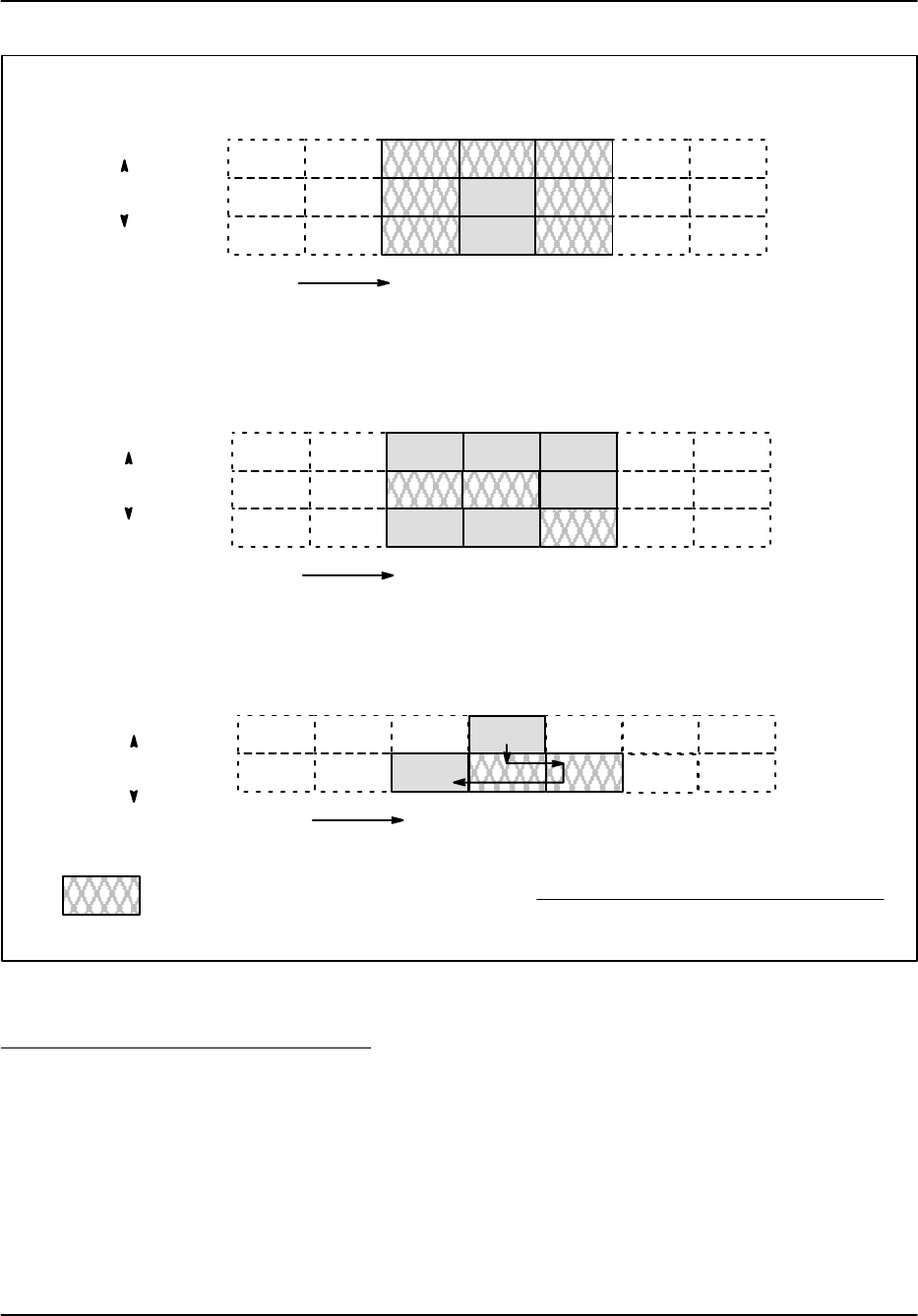
Processing Algorithms

RVP8 User’s Manual

March 2006

5–42

Range

Azimuth

-1

1-1

Zoutput

00 +Threshold

Threshold if center point is valid but there are no or only one valid neighbor.

Z00

Z0*1

Range

Azimuth

-1

1-1

Fill thresholded center point with average if there 6 or more valid neighbors.

Z0*1

Z*11 Z01

Zoutput

00 +[Z*11 )Z01 )Z11 )Z10 )Z*1*1)Z0*1]

Range

Azimuth

-1

1-1

2D Velocity Unfolding Step 1: Search pattern for valid second velocity

PRF2

PRF1

V200

V11*1

Z11

Z10

Z*1*1

Indicates Thresholded Bin

2D 3x3 Filtering Concepts

SStep 2: The unfolded velocities are then subjected to the standard 3x3 filtering.

Dual PRF, Random Phase Processing

In random phase processing, the “seam” at the start of the second trip is always problematic

since the transmitter main bang and nearby clutter will virtually always wipe out the first few

2nd trip range bins. At a constant PRF the 2nd trip seam is always at the same range, but in

dual PRF random phase mode, the seam is different each ray. Thus thresholded bins at the

seam of the high PRF can be surrounded on either side by valid bins taken at the low PRF.

The 3x3 filter has the effect of interpolating the reflectivity and width data over the bins at

the 2nd trip seam. Velocity data will also be filled–in using the nearest neighbor. Thus the

Processing Algorithms

RVP8 User’s Manual

March 2006

5–43

2D filter mitigates much of the damage that is caused at the 2nd trip seam to make a nearly

seamless display.

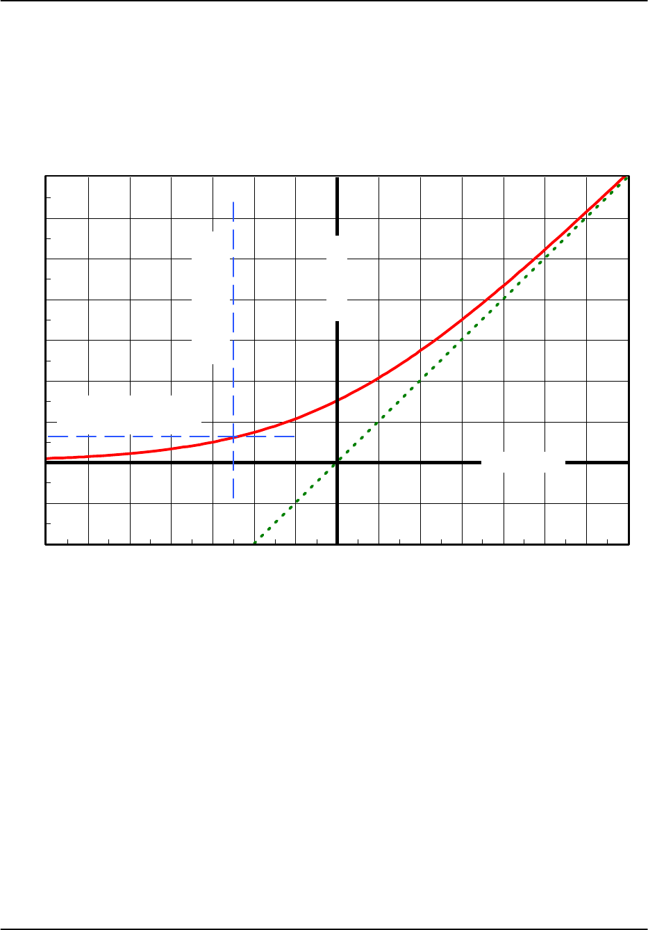
Processing Algorithms

RVP8 User’s Manual

March 2006

5–44

5.4 Reflectivity Calibration

The calculation of reflectivity described in Section 5.2.7 required the calibration reflectivity

dBZo. This section describes it’s derivation. You can use the zauto utility to perform the

calibration. (See the IRIS/RDA Utilities Manual.)

RVP8 Measured Power (2dB per Major Div)

Power at Antenna Feed (2dB per Major Division)

Figure 5–10 Model Intensity Curve

1.2dB Detection

Threshold (LOG)

10Log(Io)

–5dB SNR

Min Detectable

10Log(N)

5.4.1 Plot Method for Calibration of

This approach generates the curve shown above (red) which determines the value of Io. The

general procedure is to connect a calibrated signal generator to the radar receiver and inject

known power levels to generate a calibration plot of measured power vs the inserted power at the

antenna feed, similar to that in Figure 5–10. The calibration reflectivity dBZo is computed from

the radar constant and the value of Io, which is the intercept of the straight line fit (green) with

the Noise level.

Why does this geometric construction yield the value of Io ? Let GdB represent the overall gain

of the RF and IF components leading up to the RVP8. The green line can be interpreted as the

response of an ideal noise-free amplifier having gain GdB, while the red curve is the response of

the real-world amplifier(s) whose equivalent front-end noise is Io :

(Red) 10 log10(POUT )+GdB )10 log10(PIN )Io)

(Green) 10 log10(POUT )+GdB )10 log10(PIN )

Processing Algorithms

RVP8 User’s Manual

March 2006

5–45

The measured receiver noise is the horizontal asymptote of the red curve, i.e., the value of the

red curve when the input power PIN is zero:

10 log10(N)+GdB )10 log10(Io) .

Intersecting this measured noise level with the green straight line gives:

GdB )10 log10(Io)+GdB )10 log10(PIN )

From which we see that the input power at the point of intersection is, indeed, Io .

Note that Io is the received signal level that will produce 0dB SNR, i.e., signal power equal to

noise power. This should not be confused with the minimum detectable power PMDS which

typically will be several dB lower, depending on processor settings. In the above example, a

1.2dB LOG detection threshold is shown (horizontal blue line) for the received signal. If the

RVP8 is applying sufficient range and time averaging so that thermal noise alone produces very

few false alarms above 1.2dB, then PMDS will be a full 5dB lower than Io. We would expect a

detection rate of roughly 50% for echoes arriving at this “minimum detectable” level.

Typically a CW test signal is used to generate the test curve shown in Figure 5–10. Follow the

instructions provided by the radar manufacturer for injecting a test signal. During calibration, the

radar should be fully operational, so that all sources of noise are present. Ideally the transmitter

should be turned on during calibration.

Important: Verify with the radar manufacturer that no damage will occur to the signal

generator if the transmitter is running during the calibration.

To perform the calibration, insert signals at steps of 5 or 10 dB over the entire range of the

system. Draw the plot shown in figure 5–10. You can utilize fine resolution steps at the ends of

the scale to observer the details of the roll off. Be sure to raise the antenna up a few degrees to

avoid ground thermal noise. Also tune the frequency of the signal generator using the setup

command “pr”, and displaying the received signal spectrum. Be sure to check the tuning at the

end of the calibration to make sure the signal generator and IFD have not drifted apart.

Each time that a new signal level is injected, the measured power values are obtained by first

invoking the SNOISE command and then reading-back the results using the GPARM command.

The Log of Measured Noise Level (Word 6) from GPARM should be used. This procedure

averages many samples together. For IRIS users, this is all handled by the zauto utility.

Finally turn it all the way down and make one more sample to measure the noise level N. Io is

obtained from the intercept of the horizontal line at N and the straight line fit to the linear

portion of the curve. This value must be corrected for losses as discussed in the section below.

5.4.2 Single-Point Direct Method for Calibration of

This calibration method requires no support software. The approach uses the TTY setups

commands. Again the signal generator output must be calibrated in absolute dBm. Use a power

meter to check the calibration.

Processing Algorithms

RVP8 User’s Manual

March 2006

5–46

STurn the radiate off and connect the signal generator to the test signal injection point.

SRaise the antenna to at least 20 degrees, and set the azimuth to point away from any

known RF sources including the sun.

SSelect the pulse width using the mt command.

SSelect the pr command and use the commands to set the following:

Plotting Received Power Spectrum...

Rx:Pri, Zoom:x1–x8, Navg:25, Start:100.01 usec (14.99 km), Span:50 usec

SSet the signal generator to the approximate radar RF frequency with a power level

corresponding to a strong signal (30 dB above the noise), and use a CW signal (not a

pulse). This signal should be visible as a peak in the spectrum display. Adjust the siggen

RF signal frequency so that produces the precise IF frequency (e.g., IF frequency of 30

MHz).

STurn the signal generator off and record the “Filtered” power level. Note that because of

the large averaging it will require several seconds for the average to stabilize.

STurn the signal generator on, verify that the peak is still at the IF frequency and adjust

the power level to obtain precisely 3 dB more “Filtered” power than was observed with

the noise only. Again, allow several seconds for the averaging to stabilize after you make

each amplitude adjustment.

This is the value of Io, i.e., the test signal signal power equals the noise power. The next step is

to correct the value of Io for losses as discussed in the section below.

5.4.3 Treatment of Losses in the Calibration

In the calibration of the dBm level of the test signal, be sure to account for any losses that may

occur between the antenna feed and the injection point, and in the cable and coupler that is used

to connect the signal generator to the injection point. Figure 5–11 illustrates the nomenclature of

the various losses that are involved in the calibration. The relationship between the injected test

signal and the value of the received power relative to the feed is:

dBmFeed +dBmInjected )dBLFeed:Coupler

dBmFeed +dBmSiggen *dBLCoupler *dBLCable )dBLFeed:Coupler

For example, assume the following:

Loss between the feed and the coupler dBLFeed:Coupler 3 dB

Loss caused by the coupler dBLCoupler 30 dB

Loss in the cable from siggen to coupler dBLCable 2 dB

Then if the test signal generator output is –50 dBm, the injected power is

dBmInjected = –50–[30+2]= –82 dBm.

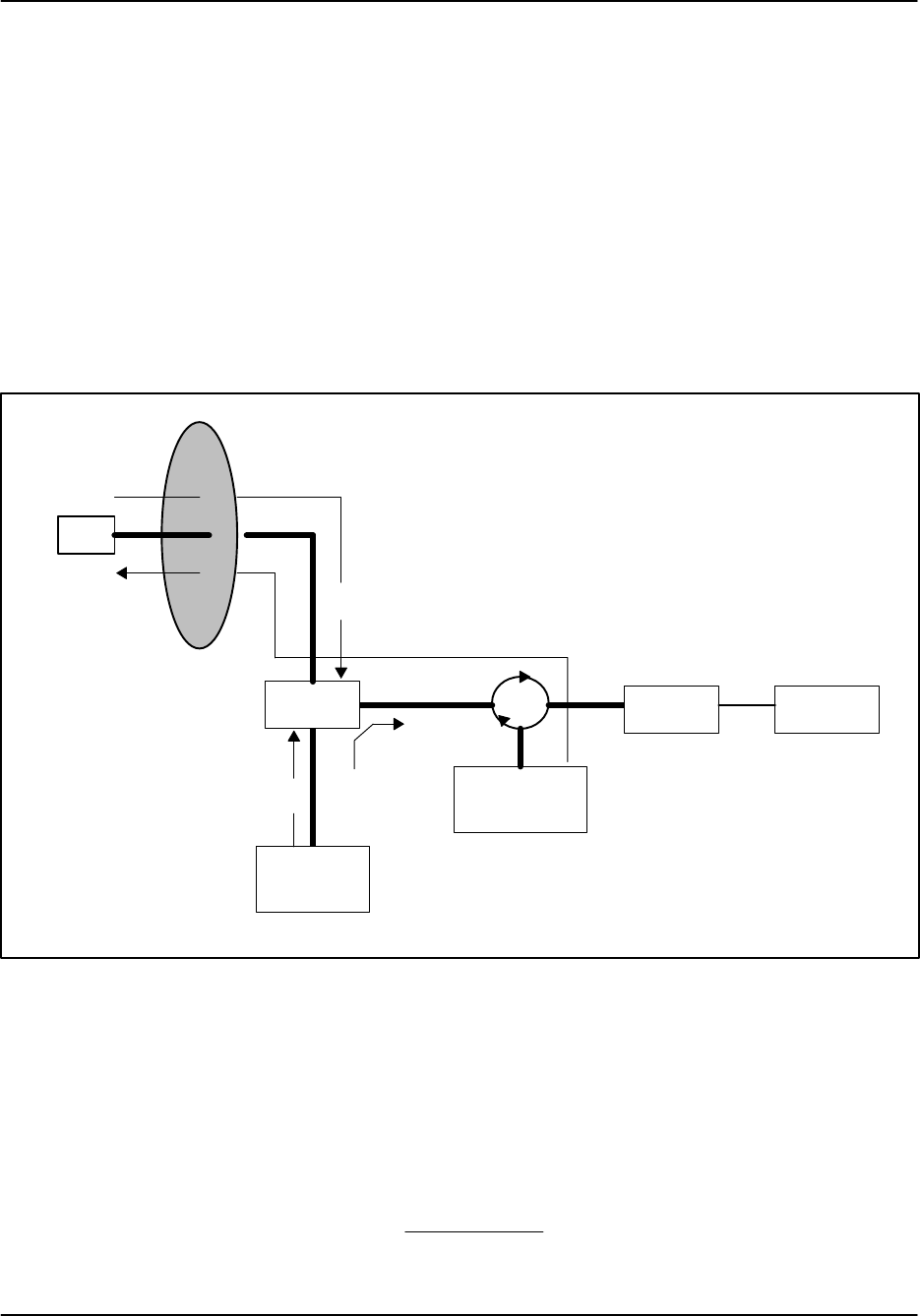
Processing Algorithms

RVP8 User’s Manual

March 2006

5–47

The equivalent power at the feed is then 3 dB more than this

dBmFeed = –82+3 = –79 dBm.

During the calibration, there are several ways to handle the losses using these equations. Two

examples are:

SEach signal generator value can be corrected for losses so that the calibration plot shows

IFD measured power vs received power at the feed. This is recommended for manual

calibration.

SThe signal generator values can be plotted directly and the intercept power Io can be

corrected for losses so that it is properly referenced to power at the feed. This is the

approach used by the IRIS zauto utility.

Figure 5–11: Illustration of Losses that Affect LOG Calibration

Transmitter

Coupler Receiver

Sig Gen

dBmsiggen

RVP7

IFD

LFeed:Coupler

Feed

Receive Path

Transmit

Path

dBmFeed

LCable

LCoupler

Pt Feed

5.4.4 Determination of

dBZ

The calibration reflectivity is determined from the radar equation as follows:

dBZo+10 log ƪCr2

oIoƫ

where Io is in mW (corrected for receive losses), the reference range ro is 1 km, and the radar

constant C is:

C+2.69 1016l2

PttqfG2Lt

Processing Algorithms

RVP8 User’s Manual

March 2006

5–48

where,

lRadar wavelength in cm.

PtTransmitted peak power in kW.

LtTransmit loss (e.g., 3 dB corresponds to Lt+2)

tPulse width in microseconds.

qHorizontal half-power full beamwidth.

fVertical half-power full beamwidth.

GAntenna gain (dimensionless) on beam axis.

The radar constant is determined from the characteristics of your radar (check with the

manufacturer if you are unsure of the values). Note that transmit losses are accounted for in the

radar constant, while receiver loss is usually included in the calculation of Io.

Finally, if the value of Io calculated above was not based on loss-corrected dBm values, correct

Io as follows:

dBIo corrected +dBIo*dBLCoupler *dBLCable )dBLFeed:Coupler

Example Calculation of

dBZo

This sample calculation is provided so that programmers can check their arithmetic. The radar

parameters:

lRadar wavelength in cm. 5 cm.

PtTransmitted power in kW. 500 kW

LtTransmit Loss 2 (3 dB)

tPulse width in microseconds 1 microsecond

qHorizontal half-power beamwidth in degrees 1 degree

fVertical half-power beamwidth in degrees 1 degree

GAntenna gain (dimensionless) on beam axis 19,953 (43.0 dB)

The radar constant for this example is,

C+2.69 1016l2

PttqfG2Lt+(2.69 1016)(5)2

(500)(1)(1)(19, 953)2(2.0)

+6.76 106ƪmm6m*3km*2mW*1ƫ

Assume that Io with loss correction is calculated to be –105 dBm (3.16 10*11 mW), then

dBZo is,

dBZo+10 logƪCr2

oIoƫ+10 logƪ(6.76 106)(1)

2(3.16 10*11)ƫ

+*36.7dB (mm6m*3)

This value would be down-loaded to the signal processor using the SOPRM command.

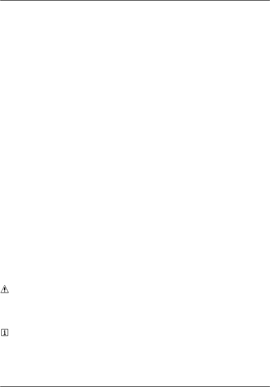
Processing Algorithms

RVP8 User’s Manual

March 2006

5–49

5.5 Dual PRT Processing Mode

The RVP8 supports two major modes for Dual PRT processing, i.e., algorithms using triggers

that consist of alternate short and long periods. Most of the Doppler parameters are available in

each of these modes. You may also request time series data in both cases; the samples will be

organized so that the first pulse of a short PRT pair always comes first.

5.5.1 DPRT-1 Mode

The DPRT-1 trigger consists of a very short PRT from which Doppler data are obtained,

followed by a much longer PRT whose purpose is to limit the average duty cycle of the

transmitter. No information is extracted from the long PRT pair, but Dual-PRF techniques can

still be used by varying the short period from ray to ray. The “-1” suffix in the name for this

mode is a reminder that Doppler parameters are computed from the short PRT only. The

DPRT-1 mode is intended for millimeter wavelength radars that must run at a very high effective

PRF (up to 20KHz) to get an acceptable unambiguous velocity, but which also have a much

lower duty cycle constraint on the average number of pulses transmitted each second.

In DPRT-1 mode the requested PRF from the host computer will generally be quite large (up to

20KHz); and the reciprocal of this “effective instantaneous PRF” will determine the trigger’s

short PRT interval. In this way, all subsequent physical calculations will be scaled correctly,

e.g., unambiguous velocity, maximum first trip range, etc., are all supposed to be based on the

short PRT interval. The host computer must therefore be configured so that it can ask for these

very high trigger rates.

The duration of the long PRT interval is not specified directly by the host computer. Rather, the

RVP8’s “Maximum number of Pulses/Second” setup parameter is used to compute how much

delay to insert in order to insure that the transmitter’s duty cycle is not exceeded. This special

treatment applies only in DPRT mode; all other modes that have uniform triggers continue to

interpret the RVP8’s trigger bound as a simple “Maximum PRF”.

Since DPRT-1 mode uses only the short pairs of pulses, it is not possible to run the “R2” moment

estimation algorithms. The RVP8 will return the GPARM “Invalid Processor Configuration” bit

if “R2” is requested in DPRT mode. The error bit will also be returned if the number of pulses

requested (sample size) is not even. All other error conditions are the same as FFT mode.

Warning: Since the RVP8’s “Maximum number of Pulses/Sec” is used to enforce

the duty cycle limit, it is essential that it not be overwritten by the host

computer’s upper PRF limit, which typically will be much higher. To insure

this, you must make sure that the PWINFO command is disabled in the RVP8

“Mc” setup menu. You will have no duty cycle protection if you do not do this.

Note: You may still choose to run Dual-PRF velocity unfolding within the

DPRT-1 mode. What will happen is that the short PRT will vary in the selected

3:2, 4:3, or 5:4 ratio, but the overall duty cycle will remain constant. The

combination of Dual–PRF and DPRT-1 is tremendously effective in extending

the radar’s unambiguous velocity interval.

Processing Algorithms

RVP8 User’s Manual

March 2006

5–50

5.5.2 DPRT-2 Mode

The trigger consists of alternating short and long period pulses, where the ratio of the periods is

determined by the velocity unfolding ratio that has been selected. Doppler data are extracted

from both the short and long pulse pairs (hence the “-2” suffix), and unfolded velocities are

made available on each ray based on the combined PRT data from that ray alone. DPRT-2 mode

is intended for rapidly scanning radars where the ray-to-ray spatial continuity assumptions of the

traditional Dual-PRF algorithms do not apply.

The DPRT-2 velocity unfolding algorithm uses a modified version of the standard Dual-PRF

algorithm. Both start by computing a simple velocity difference as a first approximation of the

unfolded result. The standard algorithm uses that difference to unfold the velocity from the most

recent ray, which yields a lower variance estimate than the difference itself. The DPRT-2

algorithm is similar, except that the folded velocity from both PRTs are unfolded independently

and then averaged together.

In addition to the above, the RVP8 also computes the DC average of the (I,Q) data within each

bin. This is used as a simple estimate of clutter power, so that corrected reflectivities are

available in DPRT-2 mode whenever a non-zero clutter filter is selected. DPRT-1 mode is the

same in this respect. However, the DPRT-2 widths use an improved algorithm based on the two

different PRTs, and which avoids the SNR sensitivity of the DPRT-1 width estimator.

Processing Algorithms

RVP8 User’s Manual

March 2006

5–51

5.6 Dual PRF Velocity Unfolding

For a radar of wavelength l operating at a fixed sampling period ts+1ńPRF , the unambiguous

velocity and range intervals are given by:

Vu+l

4ts and Ru+cts

where “c” is the speed of light. Often these intervals do not fully cover the span of velocity and

range that one would like to measure. The problem is generally worse for short wavelength

radars, since that unambiguous velocity span is directly proportional to l for a given ts. If the

unambiguous range interval is made sufficiently large by increasing ts , then the resulting

velocity span may be unacceptably small.

The RVP8 provides a built-in mechanism for extending the unambiguous velocity span by a

factor of two, three, or four beyond that given above. The technique, called Dual PRF velocity

unfolding, uses two pulse periods rather than one, and relies on the extra information thus

obtained to correct (i.e. unfold) the mean velocity measurement from each individual period.

The Dual PRF trigger pattern consists of alternating (N+k)-pulse intervals where the period in

each interval is either tl (for the low-PRF) or th (for the high-PRF). Here “N” is the sample

size, and “k” represents a delay that permits the clutter filter to equilibrate to the new PRF after

each change. The clutter filter impulse response lengths vary according to which filter is

selected.

The two trigger periods tl and th must be chosen in either a 3:2, 4:3, or 5:4 ratio. These ratios

give factors of two, three, and four times velocity expansion over the th period alone. The

unfolding algorithm makes use of the following results. Suppose that the radar observes a target

with mean velocity V at each of the two trigger periods. The measured phase angles for the R1

autocorrelations at the two PRFs are:

ql+4pVtl

l and qh+4pVth

where angles outside the basic [*p,p] interval are returned to that interval by appropriate

additions of "2p. These angles correspond to the ordinary single-PRF Doppler velocity

measurements, and the "2p uncertainties reflects the fact that each measurement is folded

into its own unambiguous interval:

Vul +l

4tl and Vuh +l

4th

If we define f to be the difference between the two measured phases then:

f+ql*qh+4p

lƪtl*thƫ

which can be interpreted as a phase angle within the unfolded interval:

Vu unfold +l

4(tl*th)

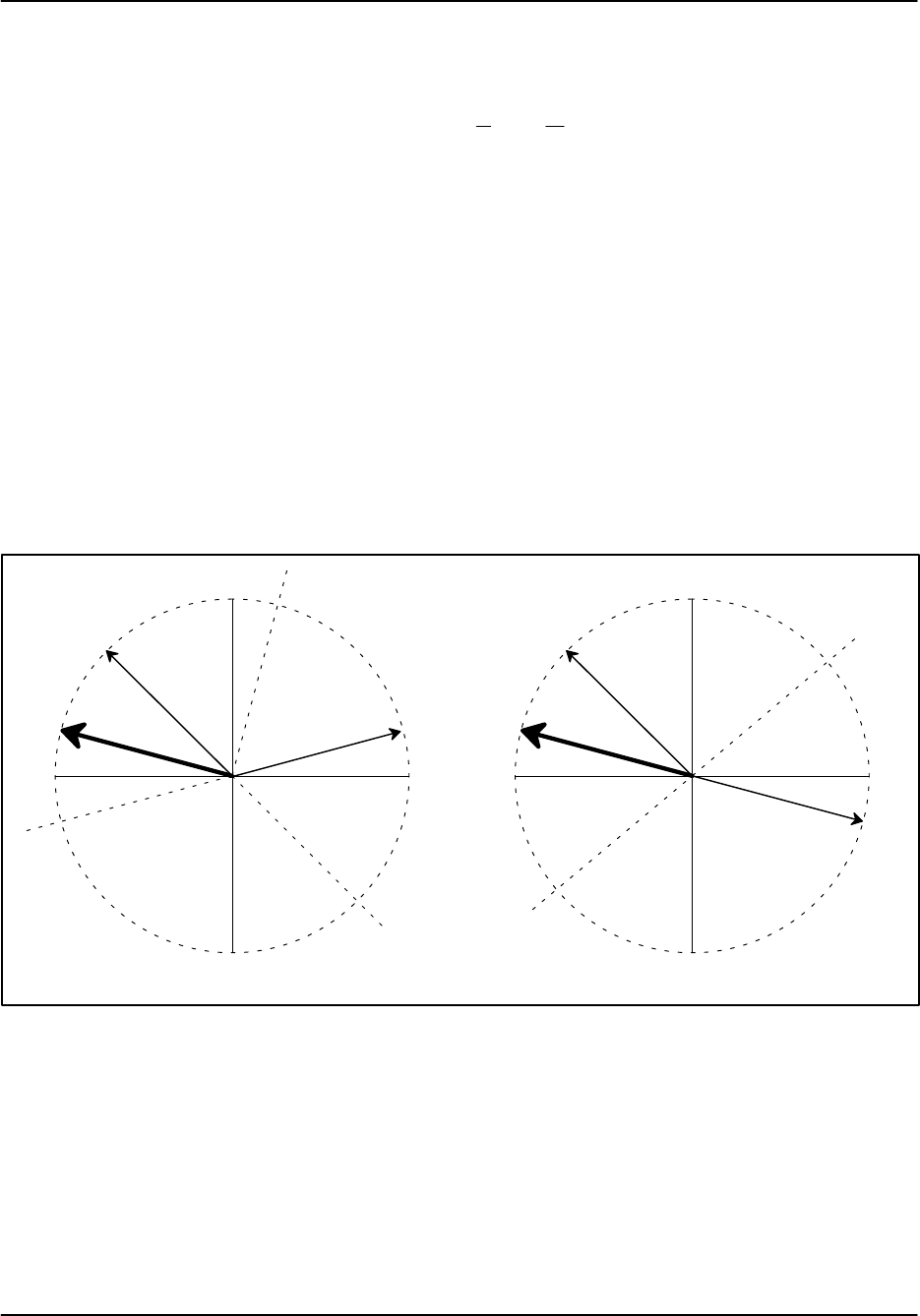
Processing Algorithms

RVP8 User’s Manual

March 2006

5–52

Now if tl and figureth are in a 3:2 ratio, then:

tl*th+tl

3+th

and thus Vu unfold +3Vul +2Vuh

The angle f represents a velocity phase angle in [*p,p] , but with respect to an enlarged

unambiguous interval. Thus, by simply differencing the folded angles from the high and low

PRFs, we obtain an angle that is unfolded to a larger velocity span. Similar reasoning shows that

the 4:3 ratio gives a factor of three improvement over Vuh , and 5:4 gives a factor of four.

In practice, the unfolded angle f is not in itself a suitable velocity estimator. The reason is that

the variance of f is equal to the sum of the variances of each of its components, i.e., twice that

of the individual measurements alone. If the target is at all noisy, then this increase in variance

can be severe. Rather than use f directly, the RVP8 uses it only as a rough estimate in

determining how to unfold the individual velocity measured from each PRF.

Figure 5–12: Dual PRF Concepts

ql*qh

Result

qlń3

Region III

Region II

Region I

Low PRF Case High PRF Case

Region I

Region II

ql*qh

Result

qhń2

This technique is illustrated in Figure 5–12. The figure shows how the low-PRF and high-PRF

angles are unfolded based on the difference angle. The diagrams show phase planes representing

the large unfolded velocity interval, and the locations of various vectors on those planes.

Referring first to the right figure, the difference angle is plotted, and the plane is divided into

two equal size regions, one of which is centered on the difference vector. The high-PRF angle is

then divided by two and plotted. The resultant unfolded velocity angle must either be this vector,

or this vector plus p. Since adding p places the vector into acceptance Region 1 where it is

Processing Algorithms

RVP8 User’s Manual

March 2006

5–53

nearest the difference angle, we conclude that this is the correct unfolding. Likewise, on the left

diagram we unfold the low-PRF angle by dividing the plane into thirds centered on the

difference angle. The result angle is either

3,ql

3)2p

3or ql

3)4p

depending on which one falls into the acceptance Region 1. Note that the resultant angle is the

same in each case.

The RVP8 makes efficient use of the incoming data by unfolding velocities from both the low

and the high-PRF data, making use each time of information in the previous ray. When low-PRF

data are taken the derived velocities are unfolded by combining information from the previous

high-PRF interval. Likewise, when high-PRF data are acquired the velocities are unfolded based

on the previous low-PRF interval. Thus, when operating in the Dual PRF mode, the RVP8

outputs one data ray for each (N+k)-pulse interval. However, the velocity data in the Dual PRF

rays are unfolded, so that the [–1,+1] interval now represents either two or three times the prior

velocity range. Put another way, the data are still interpreted as described in the section on mean

velocity estimation, except that Vu is now larger.

The width data are also modified somewhat during Dual PRF unfolding. Although valid widths

are obtained independently on all rays, those measured at low-PRF are larger than those at

high-PRF. This is simply because the dimensionless width units are with respect to a larger

velocity interval in the latter case. To compensate for this, low-PRF widths are multiplied by

either 2/3 or 3/4 before being output. This puts them in the same scale as the high-PRF values,

and thus, the widths do not vary on alternate pulses. A useful consequence of this is that width

data can be sent directly to a color display generator without having to plot every other ray in a

different scale.

There are a few words of caution that should be kept in mind when using the RVP8 in the Dual

PRF processing modes. The unfolding algorithms make the assumption that targets are

more-or-less continuous from ray to ray. Otherwise, it would not make sense to use data from a

previous ray to unfold velocities in the current ray. Users must therefore assure that their antenna

scan rate and beamwidth are such that each target is illuminated, at least partially, over each full

2(N+k)-pulse interval. In practice, a certain amount of decorrelation from ray to ray is

acceptable, since the previous rays are used only to decide into which unfolded interval the

current ray should be placed. Small errors in the previous ray data, therefore, cause no error in

the output. However, large previous-ray errors would lead to incorrect unfolding.

A more subtle side effect of Dual PRF processing arises from clutter filtering because clutter

notches now appear at several locations in the unfolded velocity span, rather than just at zero

velocity. These additional rejection points come about because the original velocity intervals are

mapped some integer number of times to create the unfolded interval. Since each original

interval has a clutter notch at DC, it follows that the final expanded velocity interval will have

several such notches. For example, in the 3:2 case, in addition to removing DC the clutter filter

removes velocities at *2Vuń3,)2Vuń3, and Vu.

Unfortunately, these clutter filter “images” are a fundamental consequence of the Dual PRF

processing technique and are not easily removed. They can cause trouble not only for the

velocity unfolding itself, but because the computed clutter corrections to be wrong at the image

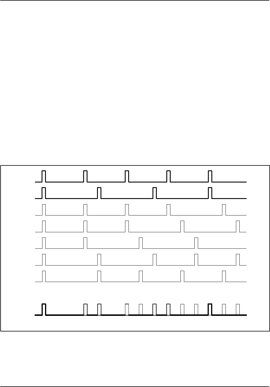
Processing Algorithms

RVP8 User’s Manual

March 2006

5–54

points. However, there is a useful work-around in the RVP8 to minimize their impact — turning

the clutter filter off at far ranges where little clutter is expected and using a narrow clutter filter

minimizes the effects of the clutter filter on weather targets.

The 4:3 and 5:4 PRF unfolding ratios are more susceptible to unfolding errors in cases where the

spectrum width is large and/or the SNR is low. The user should experiment with these ratios to

determine which provides the best results for their particular application. Although the RVP8

trigger generator can produce any trigger frequency, only the 3:2, 4:3, and 5:4 ratios can be used

with the built-in unfolding algorithms. The RVP8 still permits other PRT ratios to be explored,

but the unfolding technique must then be manually programmed on the user’s host computer.

Oscilloscope observations of Dual PRF triggers can sometimes be confusing. Figure 5–13 shows

seven possible scope traces (and their associated probabilities) for the RVP8 trigger during Dual

PRF operation. The PRF ratio is 4:3, and the sample size is 50 pulses at the high PRF, and 37

pulses at the low PRF. The signal labelled “SCOPE” is the composite of these traces, and is what

would actually be seen on an oscilloscope. Notice that there are a number of low probability pulses.

The exact details of the sample sizes and the trigger hold off time can make the low probability

pulses appear to come and go randomly. This is normal, and is no cause for alarm.

Figure 5–13: Example of Dual PRF Trigger Waveforms

47.0%

47.3%

1.0%

1.3%

SCOPE

100% 50% 50% 49% 2.3% 48.6% 48% 2.3% 2.3% 94.3% 2.3% 2.3%

Processing Algorithms

RVP8 User’s Manual

March 2006

5–55

5.7 Random Phase 2nd Trip Processing

5.7.1 Overview

Second trip echoes can be a serious problem for applications when the radar is operated at high

PRF (e.g., >500 Hz). Second trip echoes are caused by the range aliasing of targets. They appear

as false echoes on the display, usually elongated in the radial direction. On Klystron systems

they will have valid Doppler velocities. On magnetron systems, the Doppler velocities are not

valid, but the noise from the 2nd trip echoes can obscure valid first trip velocity information.

The RVP8 has optional random phase processing for the filtering and recovery of second trip

echoes. Details of the technique are proprietary to SIGMET, Inc. However, the general principle

is described here, along with a discussion of the various configuration options to optimize the

algorithm performance.

The information that is used to separate the first and second trip echoes is the phase. For a

magnetron radar, the phase of each pulse is different. This means that when 1st. and 2nd trip

echoes are received simultaneously, the phase of the first trip return is different from the phase

of the second trip return. For a magnetron radar, the RVP8 measures the phase of the transmitted

pulse and the phase locking is done digitally as opposed to the traditionally locking COHO. For

a Klystron radar, the phase is controlled by the RVP8 via a digital phase shifter that is precisely

calibrated. Typically the Klystron COHO is phase shifted so that each transmit pulse has a

different phase. The sequencing is controlled by the RVP8.

5.7.2 Algorithm

Figure 5–14 shows a schematic of the data processing for random phase. The figure shows the

Doppler spectra for the 1st. and 2nd trip in the various processing stages. The vertical scale is in

dB and the horizontal scale is velocity. In this example, the second trip echo is shown as being

stronger than the first trip echo (usually the reverse is true).

Ideal 1st and 2nd Trip Echoes

The ideal 1st and 2nd trip echoes represent the echoes as they would appear individually. The

ideal 1st trip echo is the echo that would be measured if there were no 2nd trip echo interference.

The ideal 2nd trip echo represents what would be measured if there were no 1st trip echo

interference. If there is no interference from the other trip, a standard Klystron system can

measure the ideal spectra, but there is no way to know whether the echoes are in the 1st or 2nd

trip.

Raw 1st and 2nd Trip Echoes

This figure shows how the echoes from the first trip and second trip interfere with each other.

For the case of a standard magnetron system, the first trip echo is coherent, while the second trip

echo is incoherent (white noise) since the phase of the second trip echo is random. This is

because the receiver is phase locked only to the first trip.

Processing Algorithms

RVP8 User’s Manual

March 2006

5–56

Another way to implement a magnetron system is to let the COHO free-run (rather than phase

locking to the transmit pulse), measure the phase of each transmit pulse and digitally correcting

for the transmit phase. Using this digital phase locking technique, the RVP8 can phase lock or

“cohere” to either the first or the second trip.

Using this technique alone, it is possible to distinguish between 1st and 2nd trip echoes for the

case when the echoes are not overlapped. In other words, the echoes will appear as the idealized

1st and 2nd trip echoes. This range de-aliasing effectively doubles the range of the radar. The

problem is that when echoes are overlapped, the noise contamination from the stronger echo will

make it impossible to measure the weaker echo. This is illustrated in the figure. Thus if the first

trip echo has a good signal-to-noise ratio of 10 dB, then the 2nd trip echo will have a signal-to

noise-ratio no better than –10 dB. This is the fundamental problem with using phase alone to

separate the 1st and 2nd trip echoes.

Filtered 1st and 2nd Trip Echoes

Since the strong echo generates noise that obscures the weaker echo, the approach used in the

RVP8 is to filter the echo from the other trip — the whitening filter. This is shown in the figure.

The adaptive whitening filter removes both the clutter and the weather. All of the phase

information for the other trip is then contained in the white noise portion of the spectrum. Note

that the phase information under the coherent echo that is removed will be dominated by the

coherent echo, i.e., the other trip phase information will be contaminated. For this reason, the

filtering should effect as small a region of the spectrum as possible.

5.7.3 Tuning for Optimal Performance

The Random Phase algorithms are controlled by the same collection of setup and operational

parameters that apply to all of the other processing modes, e.g., choice of sample size, clutter

filter, angle sync, calibration, etc. However, a few parameters are special to Random Phase

mode, and these are described below.

Secondary SQI Threshold

In standard Doppler processing, an SQI threshold is normally not applied to Reflectivity data

because it would cause those data to be rejected in regions of high spectral width. In Random

Phase mode we need to relax this convention because reflected power can only be assigned to a

particular trip when it is coherent within that trip. Incoherent echoes, regardless of their

strength, can not be placed into either trip.

Thus, an SQI threshold is required to qualify Reflectivity data in Random Phase mode. The

RVP8 defines a secondary SQI threshold SQI2 which is computed from the standard threshold

value simply as:

SQI2+Offset )(Slope SQI)

Where Slope and Offset are the Random Phase SQI threshold parameters defined in the Mf

setup section. The factory default values are (Slope +0.50) and (Offset +*0.05), i.e., the

secondary threshold is a little less than half of the standard value. The Random Phase

Processing Algorithms

RVP8 User’s Manual

March 2006

5–57

algorithms check whether the SQI of each recovered trip is less than the secondary SQI

threshold, and if so, the LOG portion of the data are rejected. This SQI test is necessary for a

clean LOG picture, but we need to use a more permissive (lower) threshold value than would

usually be applied to the Doppler data alone.

The Slope and Offset values should be adjusted so that the density of speckles in Random Phase

LOG data is approximately the same as the density of speckles in FFT velocity data for a given

primary SQI value. You may then adjust the primary SQI threshold to achieve the appropriate

tradeoff of speckles vs. sensitivity for your system in all modes of operation. Even with proper

adjustment, it is normal for Random Phase dBZ and dBT data to show “holes” in regions of

weather that have high turbulence or shear. These dropouts will usually match up with similar

gaps in the velocity and width data, both of which are traditionally thresholded by SQI.

Maximum Power Ratio Between Trips

The adaptive filtering that is performed on the data for each trip greatly extends the visibility of

a weak echo that is overlapped with a much stronger one. In practice, the filtering process is

often able to remove 25-35dB of dominant power in order to reveal a much weaker echo in the

other trip. The performance depends on many factors, primarily the spectral width of the

dominant echo, and the overall stability of the radar system.

The difficulties of removing a dominant “other trip” echo from a weather signal are analogous to

the challenge of removing a dominant clutter target from that same signal. In both cases we are

trying to extract a weak weather signature using a filtering procedure that relies on the spectral

confinement of the stronger signal. The RVP8 already has a parameter that can be adjusted to

control sub-clutter visibility, i.e., the Clutter-to-Signal Ratio (CSR). Just as the CSR applies to

the clutter filters, it can likewise be used to place similar limits on the depth of visibility of the

adaptive filters.

As an example, suppose that the RVP8 is operating in Random Phase mode at a PRF of 1500Hz,

and is observing widespread weather having uniform intensity in both the first 100Km trip and

the second 100Km trip. If the CSR were set too conservatively at only 15dB, then the algorithm

would generally be blind to second-trip weather in the range interval from 100km to 117.8km.

The explanation for this can be found in the 1ńr2 geometric correction for weather echo

intensity. At ranges less than 17.8km, the first trip weather would generally dominate the second

trip weather by more than 15dB. Thus, the initial 17.8km ring of second trip data would be

rejected by the CSR criteria. However, if the CSR were increased to 30dB, then the size of this

missing ring would be reduced to only 3.2km.

If the CSR is set too low you will notice an abrupt ring of missing data in the beginning of the

second trip. If set too high, there will be speckles and other spurious effects within this same

interval. The optimum setting should strike a balance between these two effects.

R1 vs. R2 Algorithms

The Random Phase algorithms for adaptive filtering and separation of trips relies on having the

best possible information about the weather’s SNR and spectral width. Thus, the “R2” Doppler

algorithms are always used, regardless of the setting of the R1/R2 flag in the user’s operational

parameters.

Processing Algorithms

RVP8 User’s Manual

March 2006

5–58

Random Phase and Dual PRF

The random phase processing works seamlessly with the dual PRF processing to provide

advanced range and velocity ambiguity resolution. Both the first and 2nd trip echoes can be

recovered and displayed to a maximum range of 2X the unambiguous range corresponding to the

high PRF.

For optimum performance, the 2D 3x3 speckle filter should be used to smooth the 2nd trip

seams that occur for each ray. In fact, this smoothing of the 2nd trip seam makes the dual PRF

random phase mode work even better than the single PRF random phase.

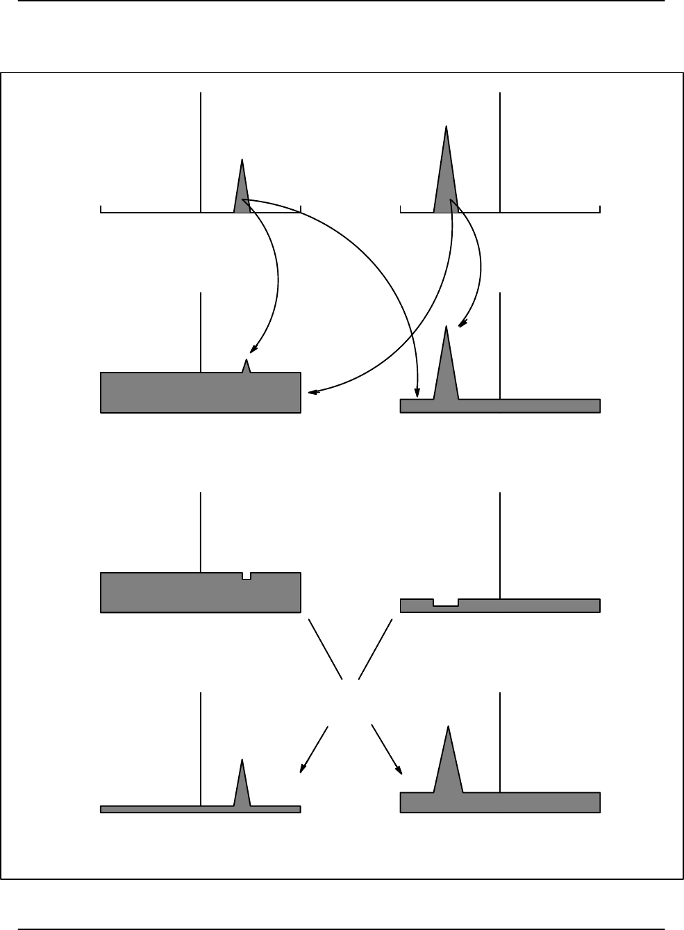
Processing Algorithms

RVP8 User’s Manual

March 2006

5–59

Figure 5–14: Random Phase Processing Algorithm

Ideal 1st Trip Ideal 2nd Trip

Raw 1st Trip with Raw 2nd Trip with

Filtered 1st Trip Filtered 2nd Trip

Inverse Transfrom

2nd Trip Noise Contamination 1st Trip Noise Contamination

and ReĆCohere

Recovered 1st Trip Recovered 2nd Trip

Processing Algorithms

RVP8 User’s Manual

March 2006

5–60

5.8 Signal Generator Testing of the Algorithms

This section describes a variety of IF signal generator tests that can be used to verify correctness

of the RVP8 processing algorithms. These tests are routinely performed at SIGMET whenever

new algorithms and/or major modes are added to the processor. We have include a few of the

test descriptions here so that they can be used by customers who need to debug their systems, or

who want to better understand how they work. Additional tests for receiver sensitivity and

dynamic range can be found in Appendix D.

5.8.1 Linear Ramp of Velocity with Range

Suppose that a continuous-wave IF waveform has an instantaneous frequency f(t) in Hertz

(cycles/sec). Consider a range bin located at time tbin within a set of pulses that are separated by

ts+1ńPRF. The phase measured at that bin on the nth pulse will be the integral of the frequency

within that pulse starting from range zero (since the RVP8 is phase locked to range zero):

Fn+ŕ

nts)tbin

nts

f(t)dt

If we assume that the input frequency is a linear Frequency Modulation (FM) at the rate of M

cycles/sec/sec on top of a base frequency To, then:

Fn)1*Fn+ŕ

(n)1)ts)tbin

(n)1)ts

(To)Mt)dt *ŕ

nts)tbin

nts

(To)Mt)dt +(Mts)tbin

which, remarkably, is independent of both To and n. Thus, a linear FM input signal produces a

fixed (I,Q) phase difference from pulse-to-pulse at any given range. The magnitude of the phase

difference is proportional to the range, and the slope is (ĂMĂtsĂ) cycles for each second of delay in

range. For example, if the test signal generator is sweeping 100KHz every two seconds, then the

velocity observed at a range of 300km at 250Hz PRF will be:

Fn)1*Fn+ǒ100 KHz

2 sec Ǔ ǒ1

250 sec Ǔ (300 km ) ǒ6.6 msec

1km Ǔ+0.40 cycles

We would thus observe a velocity of (0.8 Vu) at 300km, where VuĂ is the unambiguous

Doppler velocity in meters/sec. Note that these phase difference calculations have made no

assumptions about the RVP8 processing mode, and thus are valid in all major modes (PPP, FFT,

DPRT, RPH), as well as in all Dual-PRF unfolding modes.

Interestingly, this simple FM signal generator will also produce valid second trip velocities that

can be seen during Random Phase processing. This follows from the above analysis because

we’ve never assumed that tbin was smaller than ts, i.e., it is fine for the range bin to be located

in any higher-order trip.

Processing Algorithms

RVP8 User’s Manual

March 2006

5–61

5.8.2 Verifying PHIDP and KDP

The PHIDP and KDP processing algorithms can be tested using CW signal sources at IF. In the

alternating-transmitter single-receiver case, a single FM signal generator is modulated with an

RVP8 polarization select line so that slightly different frequencies are generated for the H and V

pulses. A maximum FM depth of several kilohertz is all that is required. In the dual-receiver

case, two (unmodulated) signal generators are used for each of the H and V intermediate

frequencies, and one or the other is detuned slightly from its correct center frequency. In either

case the frequency difference that produces a KDP value of 1.0 degree/km will be:

(1.0 degree

km ) (1

360

cycles

degree ) ( 299792 km

second )+833 cycles

second

5.8.3 Verifying RHOH, RHOV, and RHOHV

These three terms measure the normalized cross-channel covariance in a polarization radar.

They all are computed in essentially the same way having the form:

RHOAB +tsn

Asn

B*u

ts2

Aut s2

Where the sn

A and sn

B are complex (I,Q) vectors from two receiver channels A and B, and “<>”

denotes expected value. This suggests that some form of amplitude modulation (AM) of the

input signal might be helpful.

Suppose that the sn

A and sn

B samples are coming from two signal generators installed on a

dual-receiver system, and that only the B-Channel is AM modulated so that:

|sn

A|+{S

A,SA,SA,SA,SaAAA },|sn

B|+{S

B,0,SB,0,SBAAA }

Then the above estimator reduces to:

RHOAB +(1

2)SASB

A (1

2)S2

Ǹ++0.707

A simple way to create these data is to set the A-Channel siggen for 95% AM depth, and use a

sinusoidal modulation source of, perhaps, 400Hz. The reason for not choosing 100% depth is

that we would loose the Burst phase reference when the amplitude became smallest. The 26dB

reduction in SB is a close enough approximation to zero in the above formula.

If we now observe the two receive channels with the RVP8 at a PRF of 800Hz, we will see the

various RHOAB terms varying with range; reaching a high value of 1.00, and a low value of

0.707. The plots will be nearly stationary on the ascope screen because the PRF is almost

precisely twice the modulation rate (though they are free-running relative to each other).

Adjusting the amplitude of either signal generator will not affect the ò terms, but it will have an

interesting effect on SQI. If (T,Z,V,W) are being computed from both channels combined, then

the SQI is:

SQI +S2

A)(1

2)S2

Processing Algorithms

RVP8 User’s Manual

March 2006

5–62

If we solve this equation for SQI=0.5 we find that the individual SA terms must have twice the

power of the individual SB terms. This can be checked by adjusting either signal generator until

the minimum plotted SQI is 0.5, and then verifying that the average H and V powers are

identical; or, equivalently, that ZDR, LDRH and LDRV are zero.

The linear FM ramp described in Section 5.8.1 can also be used as a test of RHOAB in a

dual-receiver system. With one siggen modulated and the other fixed, one receive channel will

appear to be rotating relative to the other. If the FM modulation is such that 1/N of a full

revolution occurs per pulse at a given range, then if the sample size is N pulses we will observe

RHOAB +0 at that range. In fact, the plot of RHOAB will show a characteristic sin(x)ńx behavior

as a function of range.

Baron Services DSSR-250C Pulsar Digital Solid-State Radar System User Manual

Baron Services Inc Pulsar Digital Solid-State Radar System

Contents

Processing Algorithms

Navigation menu

Namespaces

Views

Navigation