Baron Services DSSR-250C Pulsar Digital Solid-State Radar System User Manual
Baron Services Inc Pulsar Digital Solid-State Radar System
UserManual.wiki
>
Baron Services
>
DSSR-250C User Manual
>
Processing Algorithms
Contents
1.
Users Manaul Cover Page and Table of Contents
2.
Hardware Limited Warranty
3.
Introduction and Specifications
4.
Hardware Installation
5.
Plot Assisted Setups
6.
Processing Algorithms
7.
TTY Nonvolatile Setups
8.
Host Computer Commands
Processing Algorithms
Navigation menu
Upload a User Manual
Namespaces
Wiki Guide
HTML
PDF
Info
Views
User Manual
Discussion / Help
Navigation
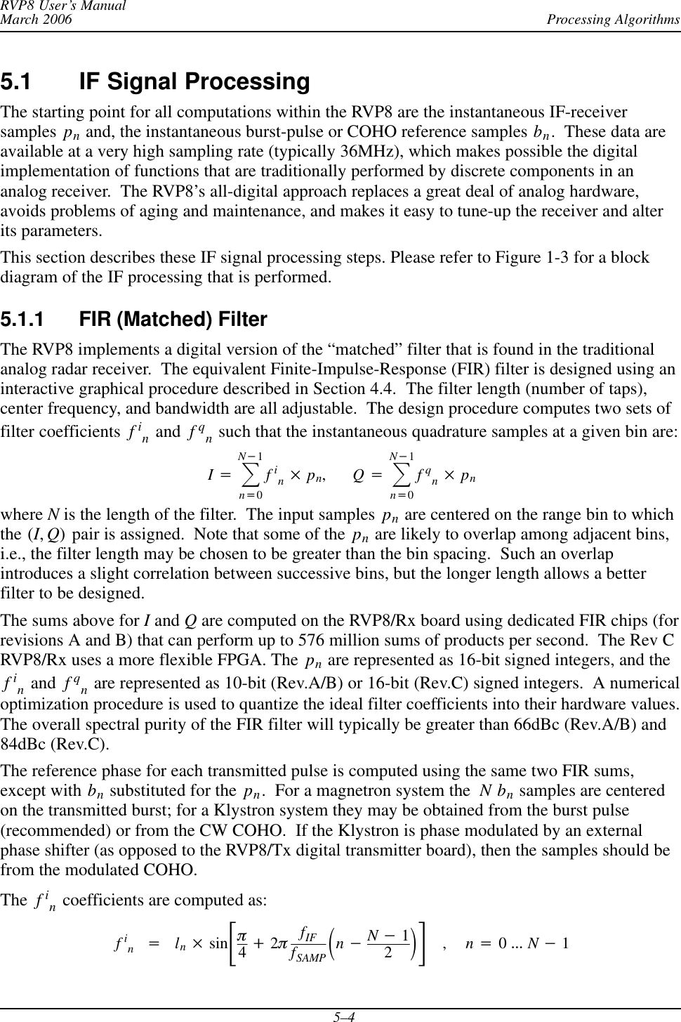
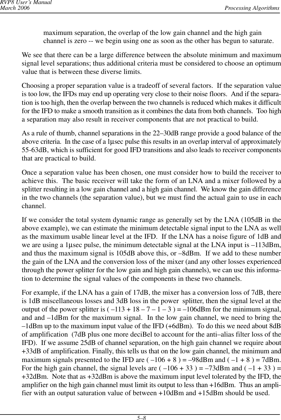
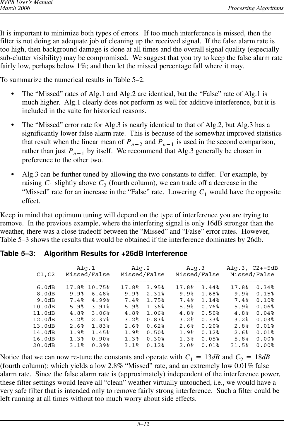
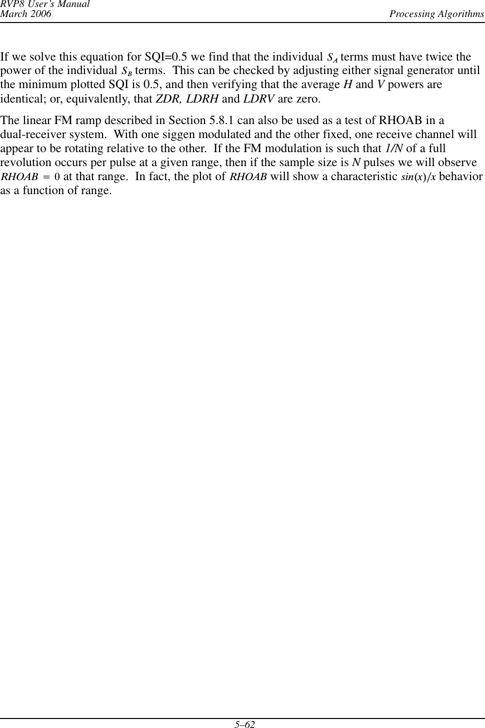
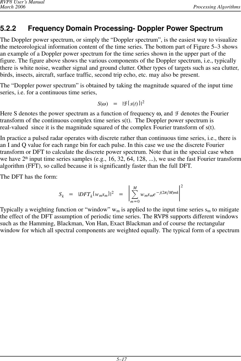
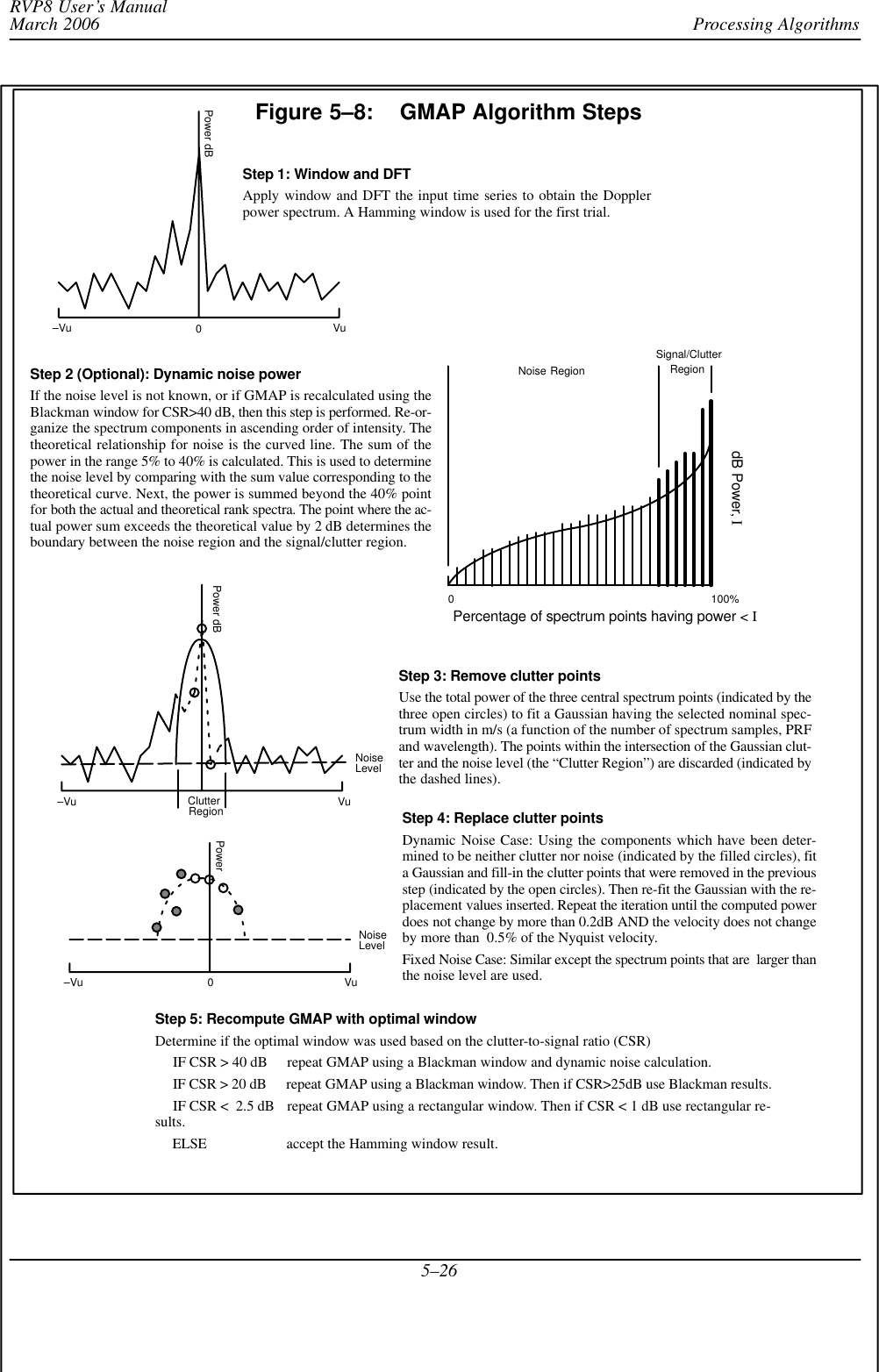
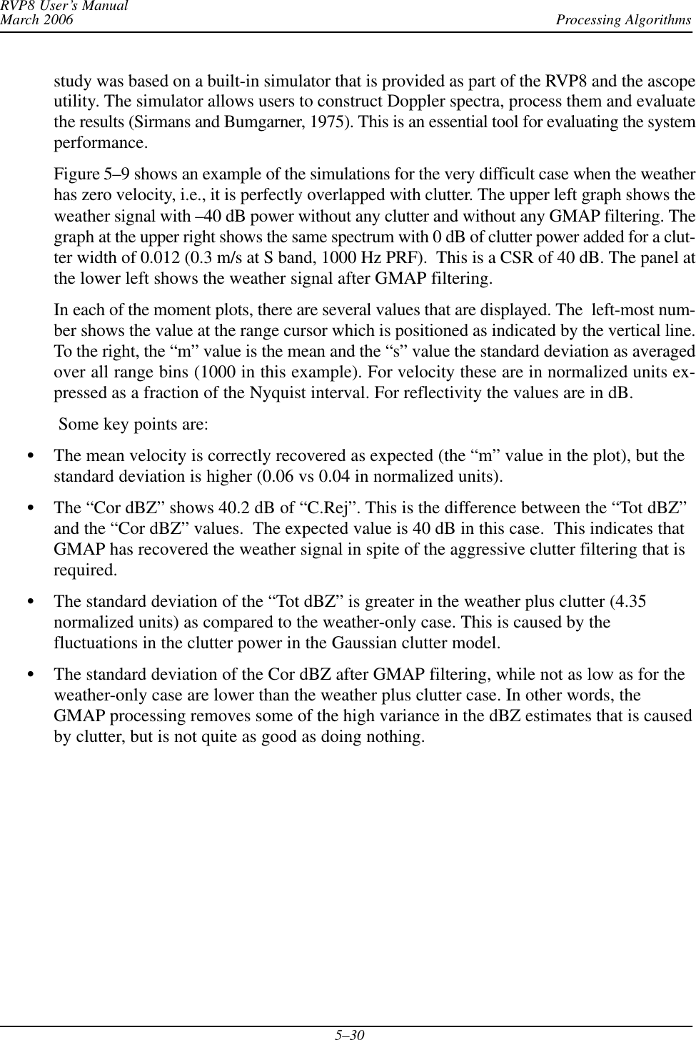
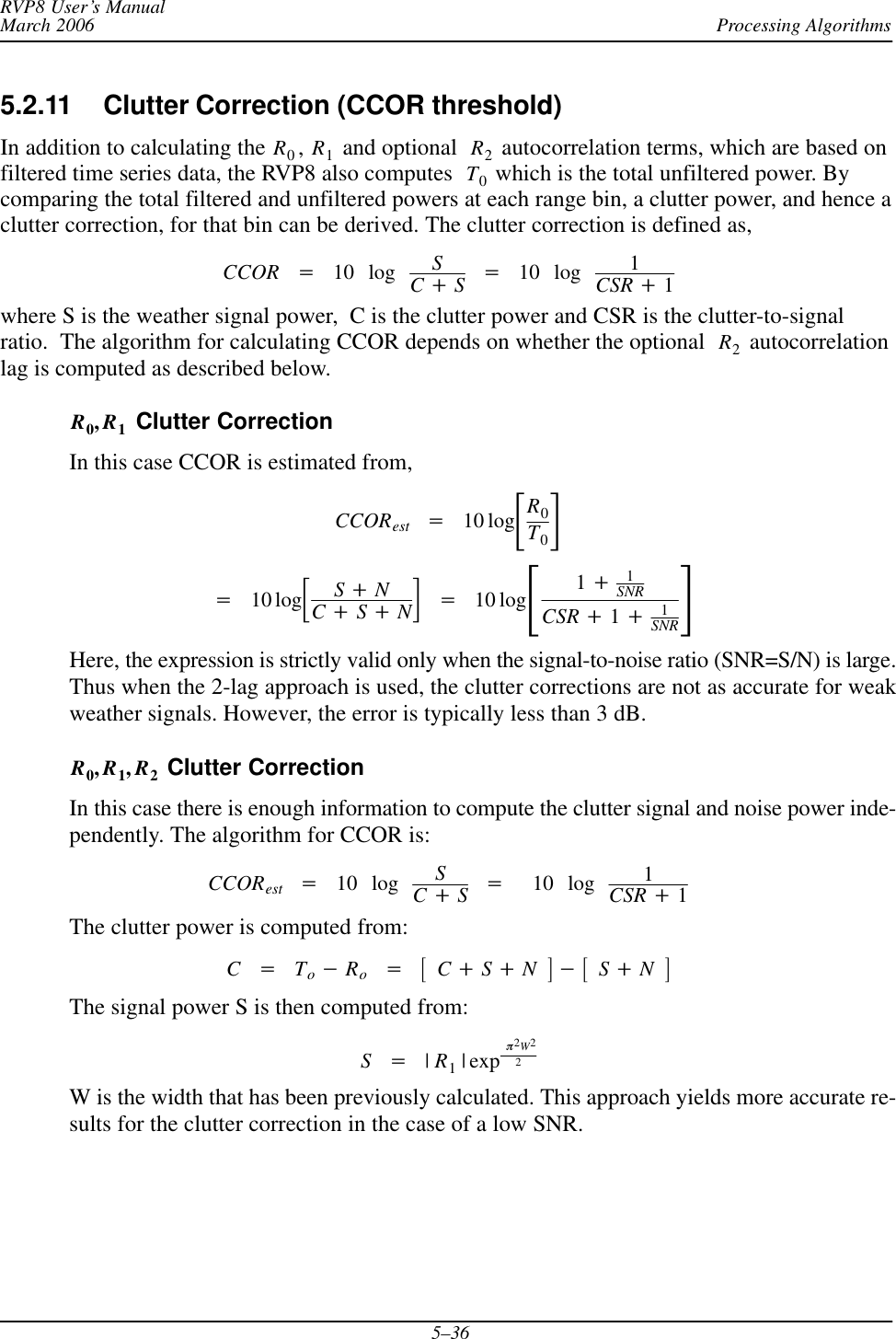
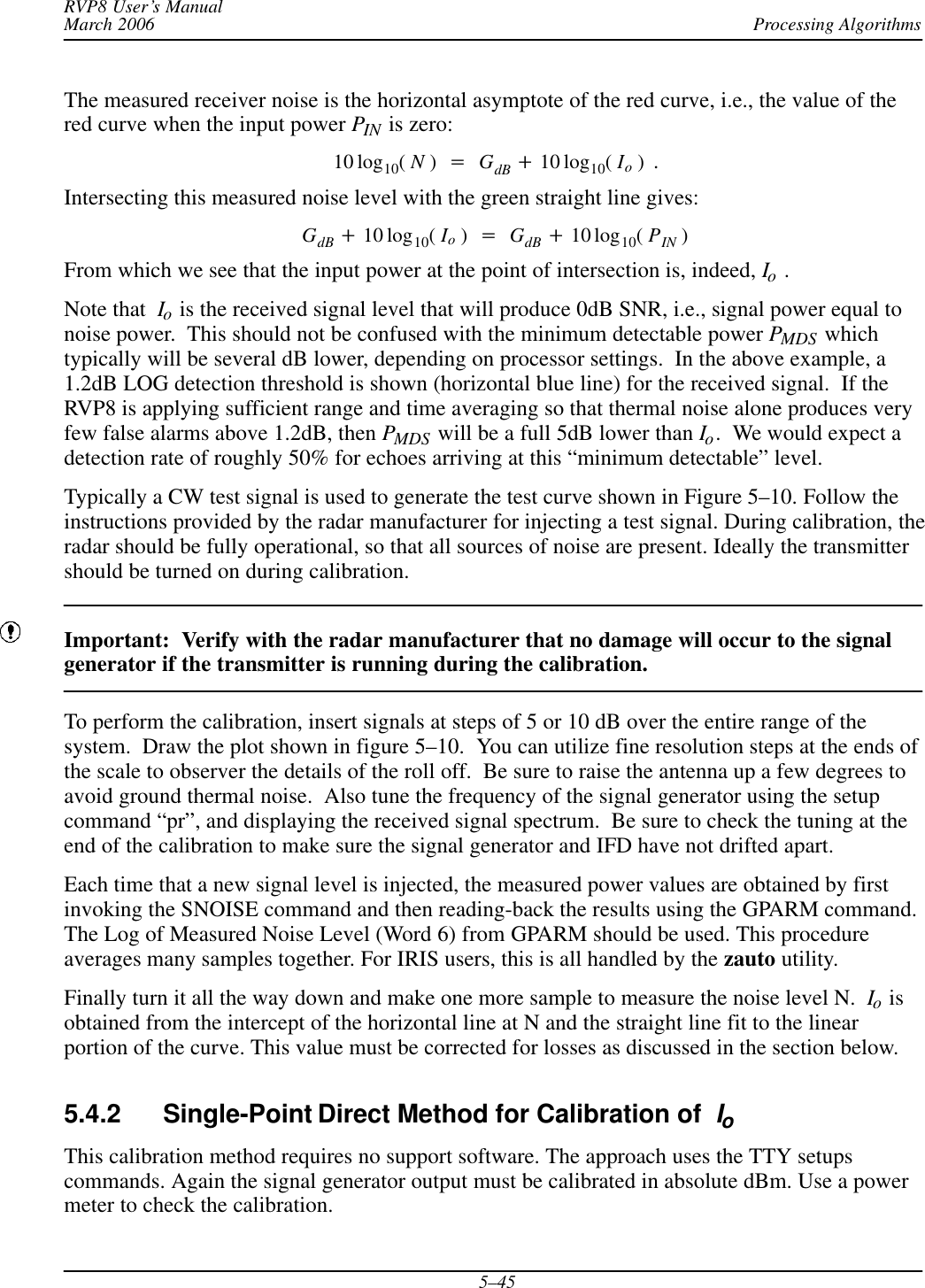
![Processing AlgorithmsRVP8 User’s ManualMarch 20065–155.2 Time Series (“I” and “Q”) Signal Processing5.2.1 Time Series Processing OverviewThis section describes the processing of the radar time series data (also called linear “video” or“I” and “Q”) to obtain the meteorologically significant “moment” parameters: reflectivity, totalpower, velocity, width, signal quality index, clutter power correction, and optional polarizationvariables.Recall that the time series synthesized by the FIR filter consist of an array of complex numbers:sm+[Im)jQm]for m+1, 2, 3, AAA,Mwhere “j” is *11ń2. The time series, are the starting point for all calculations performedwithin the RVP8. There are several excellent references on the details of I and Q processing. Thereader is referred to Doviak and Zrnic’s text on the subject. The top part of Figure 5–3 shows Iand Q values for a simulated time series using the ascope utility.There are two broad categories of time series signal processing:STime Domain Processing using the I and Q samples directly to calculate“autocorrelations” and then using the autocorrelations to compute the moments. This isused by many systems since the algorithms are very efficient requiring minimal storageand computational power. However, time domain algorithms are generally not adaptiveor very flexible.SFrequency Domain Processing using the I and Q samples to calculate a Doppler powerspectrum and then applying algorithms, such as clutter filtering or 2nd trip echofiltering/extraction, in the frequency domain. The Doppler spectrum is then inverted toobtain the autocorrelation functions and these are used to calculate the moments. Thefrequency domain is well suited to more complex adaptive algorithms, i.e., where theprocessing algorithm is optimized for the data.The RVP8 supports the concept of “major modes” or processing modes to process the timeseries. Currently the following major modes are supported by SIGMET:SDFT/FFT Mode is a frequency domain approach which is used for most operationalprocessing applications. There are a variety of clutter filtering options, including theGMAP algorithms (Gaussian Model Adaptive Processing).SPulse Pair Processing or PPP Mode is a time domain approach that is used primarily fordual polarization applications.SRandom Phase Mode or RPHASE is a frequency domain approach similar to theDFT/FFT, except that filtering and extraction of both the first and second trip echoes issupported.SBatch Mode during which a small batch of low PRF pulses is transmitted (e.g., for 0.1degree of scanning) followed by a large batch of higher PRF pulses (e.g., for 0.9 degreesof scanning) to determine which ranges are likely contaminated by second trip echo. This](https://usermanual.wiki/Baron-Services/DSSR-250C.Processing-Algorithms/User-Guide-669147-Page-15.png)
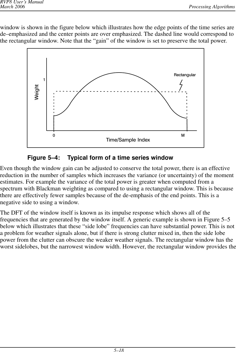
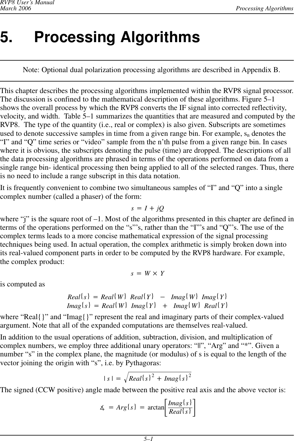
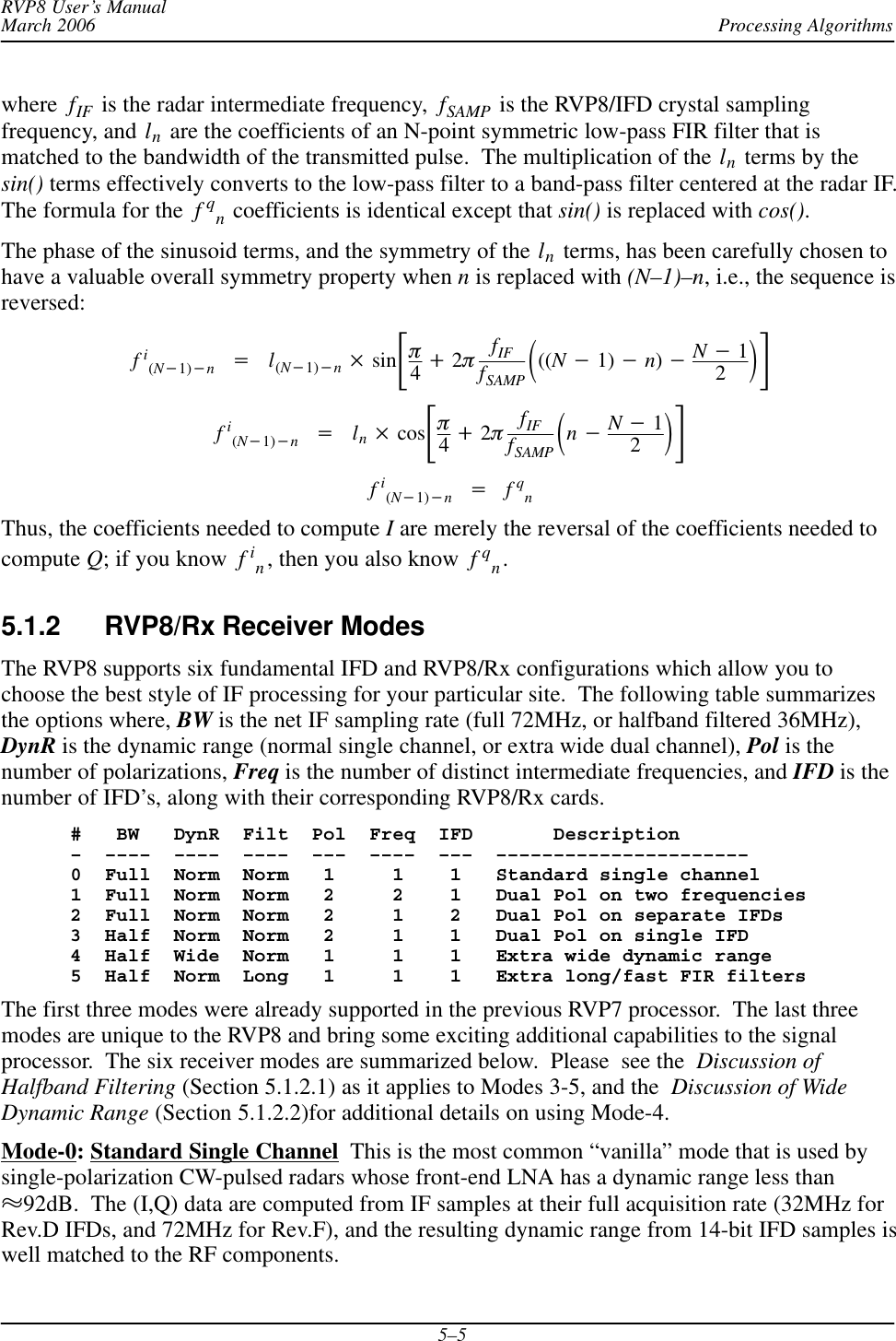
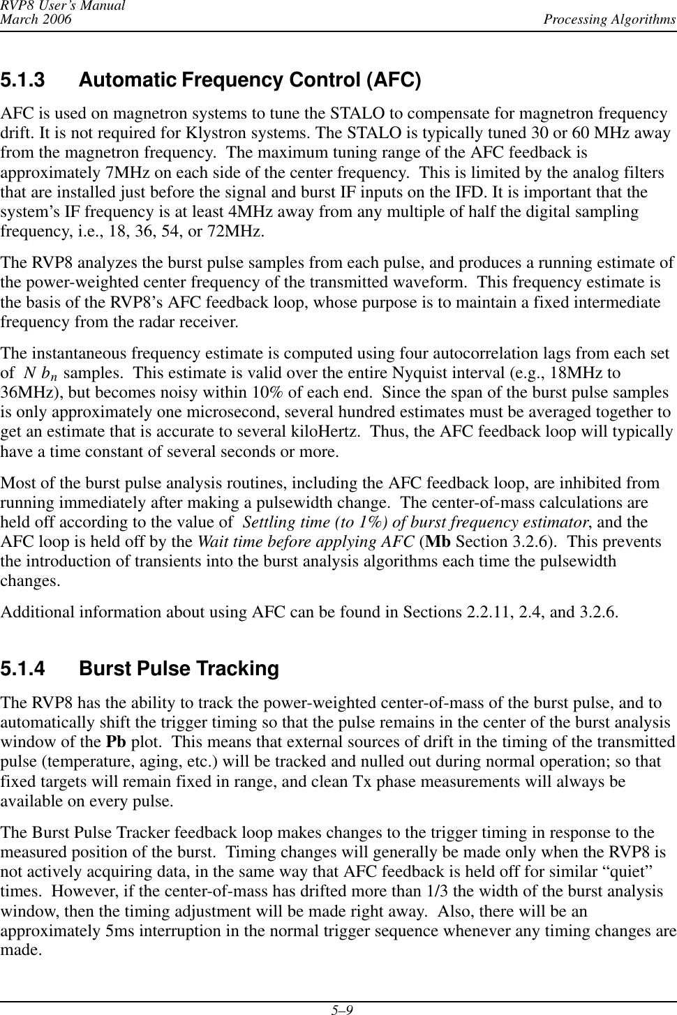
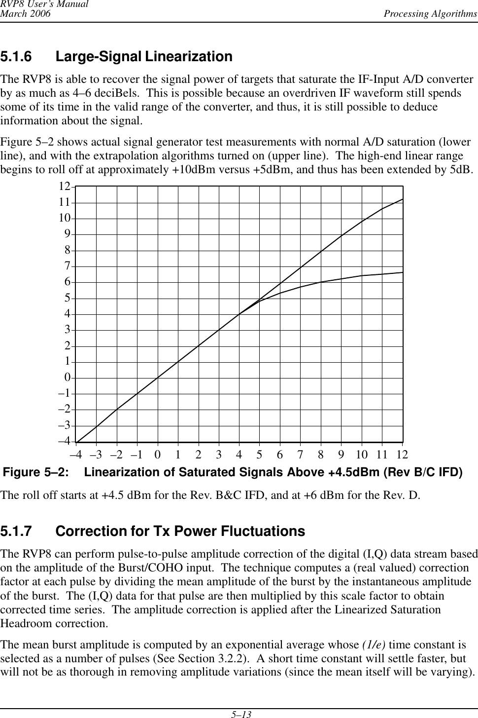
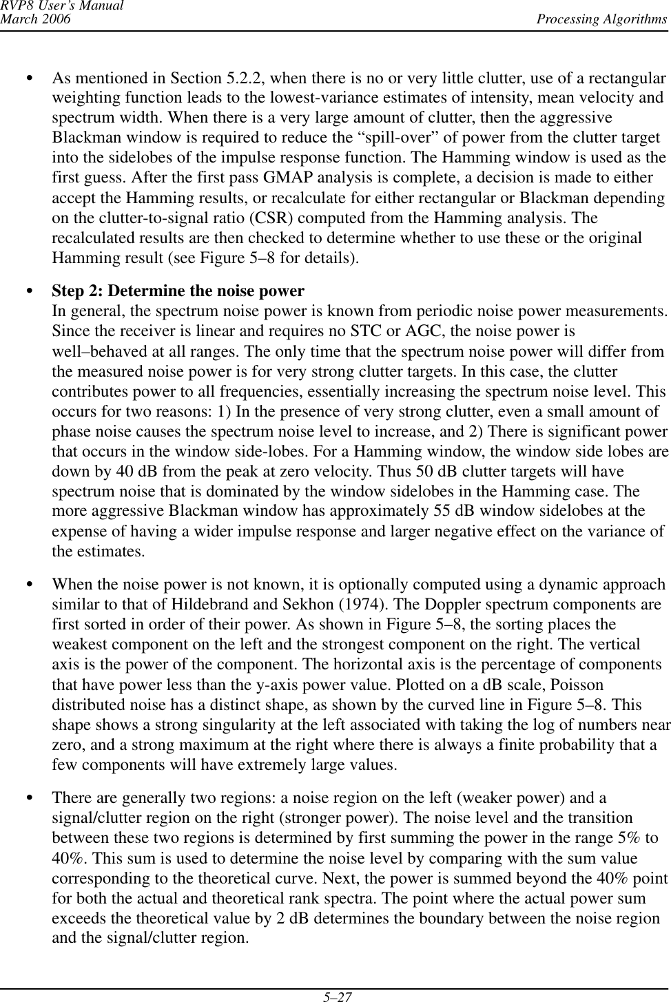
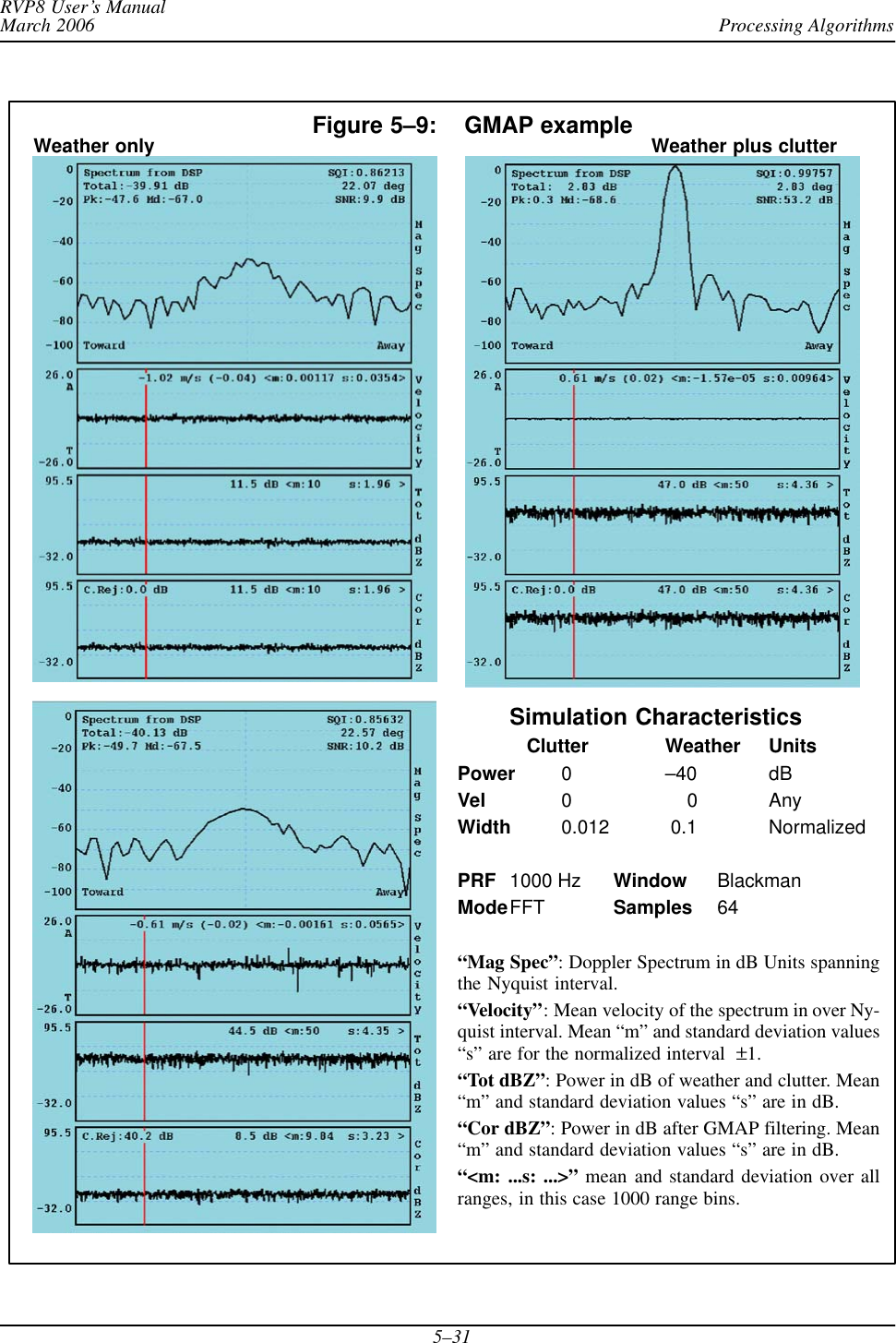
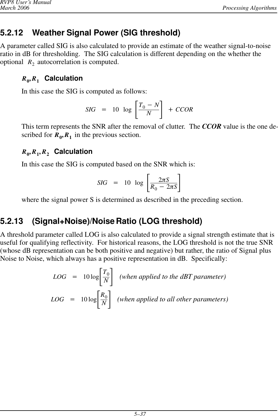
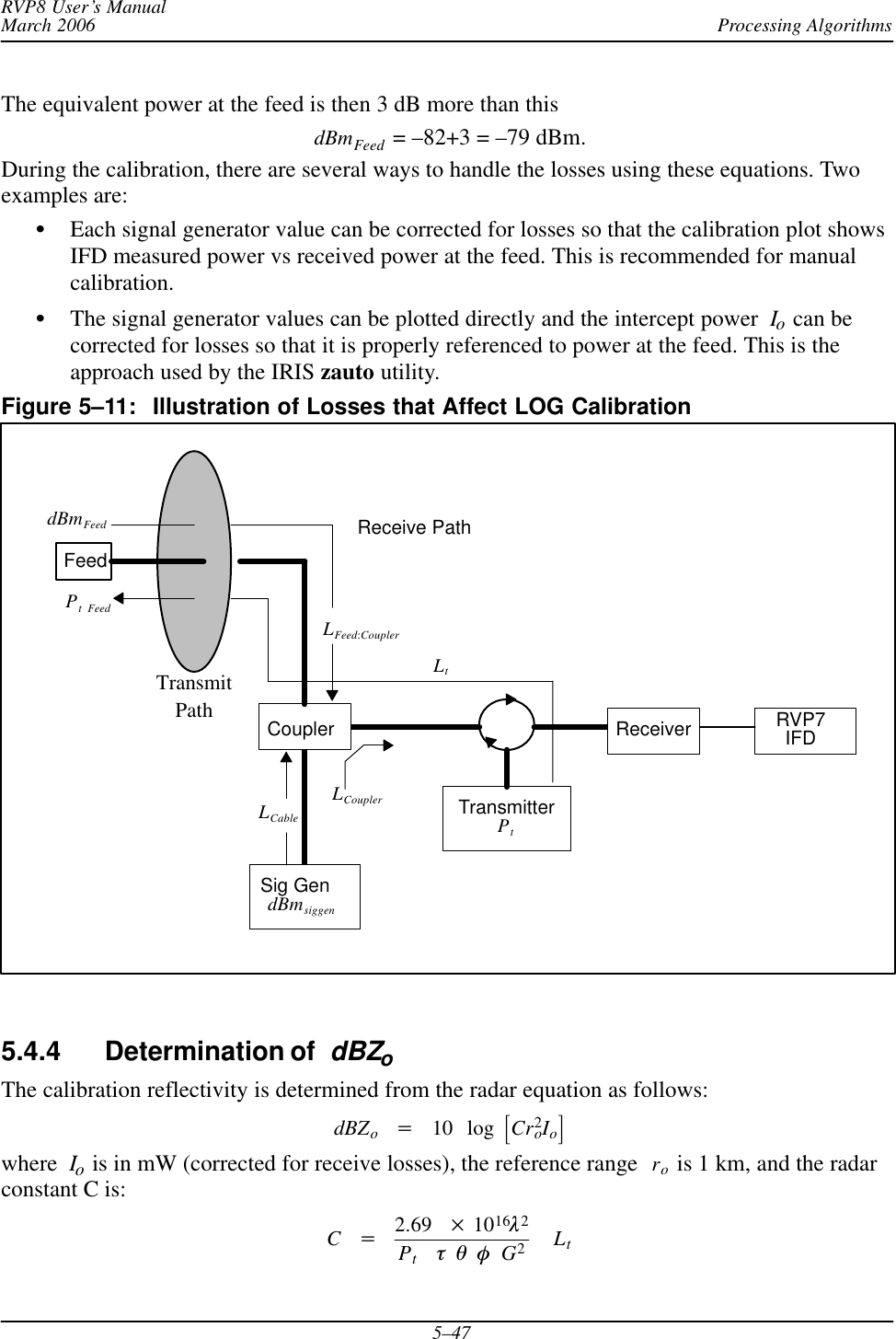
![Processing AlgorithmsRVP8 User’s ManualMarch 20065–205.2.3 AutocorrelationsThe final spectrum moment calculation (for total power or SNR, mean velocity and spectrumwidth) in all processing modes is based on autocorrelation moment estimation techniques.Typically the first three lags are calculated, denoted as R0, R1 and R2. However, there are twoways to calculate these, i.e., time domain or frequency domain calculation. In the PPP mode fordual polarization, the autocorrelations are computed directly in the time domain while in theDFT mode, they are computed by taking the inverse DFT the Doppler power spectrum in thefrequency domain. Note that only the first three terms need be calculated in the inverse DFTcase. The time domain and frequency domain techniques are nearly identical except that themethod of taking the inverse DFT of the power spectrum relies on the assumption that the timeseries is periodic. Another difference is that for time domain calculation only a rectangularweighting is used.The time domain calculation of the autocorrelations and the corresponding physical models are:Parameter and Definition Physical ModelTo+1MȍMn+1sn*sngrgt(S)C))NRo+1MȍMn+1sȀ*nsȀngrgtS)NR1+1M*1ȍM*1n+1sȀ*nsȀn)1grgtSejpVȀ*p2W2ń2R2+1M*2ȍM*2n+1sȀ*nsȀn)2grgtSej2pVȀ*2p2W2where M is the number of pulses in the time average. Here, sȀ denotes the clutter-filtered timeseries, s denotes the original unfiltered time series and the * denotes a complex conjugate. gr andgt represent the transmitter and receiver gains, i.e., their product represents the total system gain.Since the RVP8 is a linear receiver, there is a single gain number that relates the measuredautocorrelation magnitude to the absolute received power. However, since many of thealgorithms do not require absolute calibration of the power, the gain terms will be ignored in thediscussion of these. To for the unfiltered time series is proportional to the sum of themeteorological signal S, the clutter power C and the noise power N. R0 is equal to the sum ofthe meteorological signal S and noise power N which is measured directly on the RVP8 byperiodic noise sampling. To and R0 are used for calculating the dBZ values- the equivalent radarreflectivity factor which is a calibrated measurement. The physical models for R0,R1 and R2correspond to a Gaussian weather signal and white noise as shown in Figure 5–3. W is thespectrum width and V’ the mean velocity, both for the normalized Nyquist interval on [–1 to 1].The autocorrelation lags above and the corresponding physical models have five unknowns: N,S, C, V’, W. Because the R1 and R2 lags are complex, this yields, effectively, five equations infive unknowns using the constraint provided by the argument of R1. This closed system ofequations can be solved for the unknowns which is the basis for calculating the moments fromthe autocorrelations.](https://usermanual.wiki/Baron-Services/DSSR-250C.Processing-Algorithms/User-Guide-669147-Page-20.png)
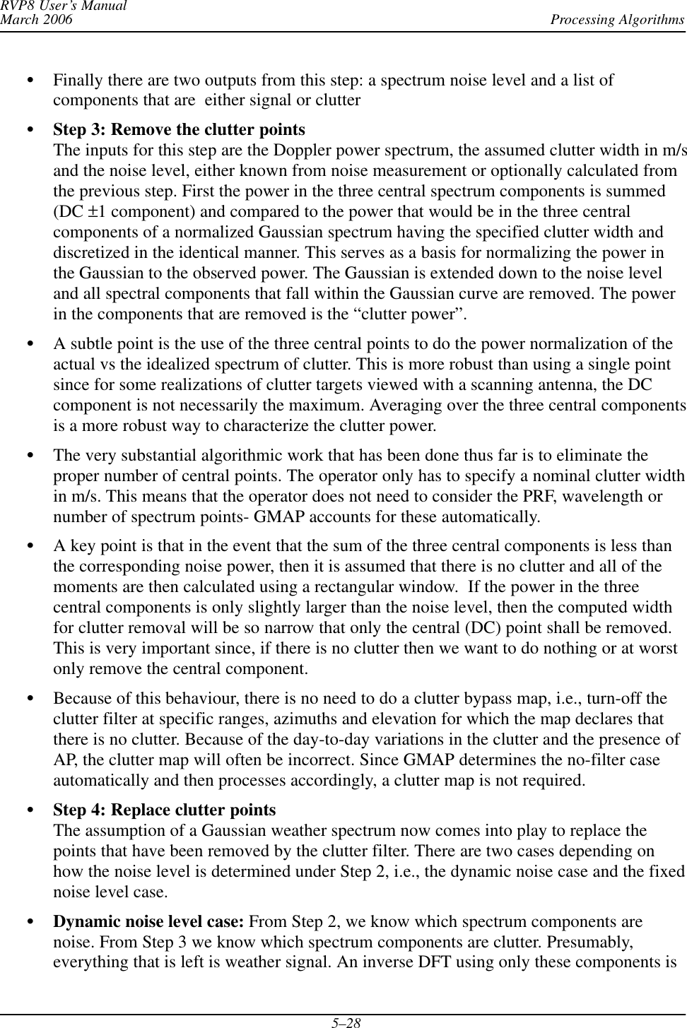
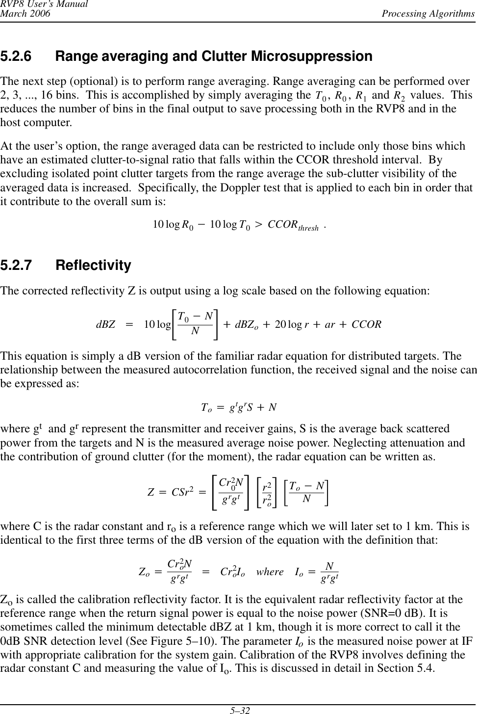
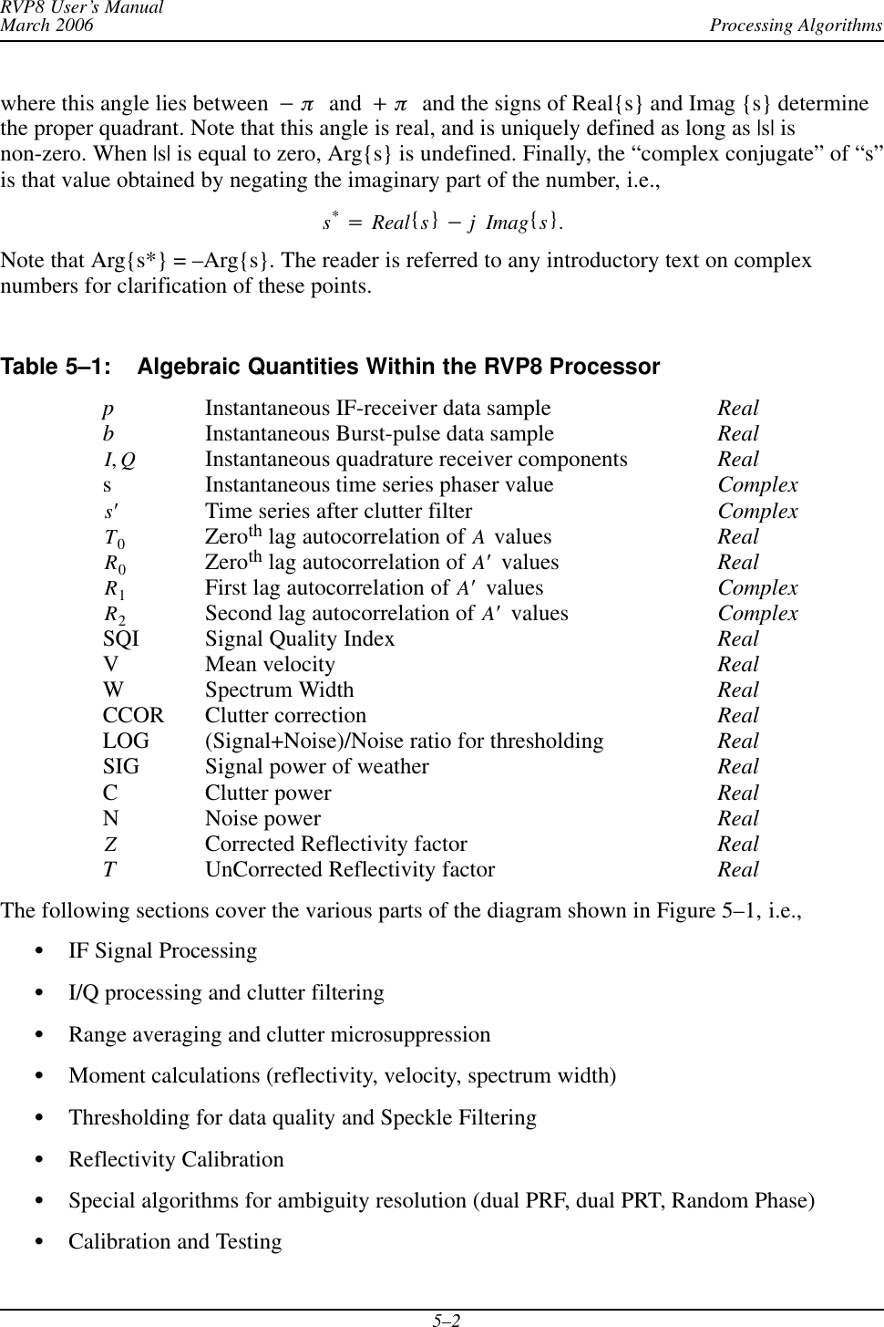
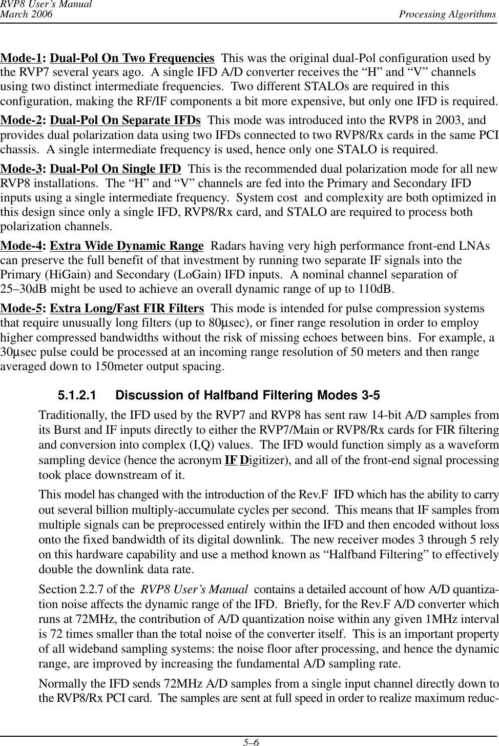
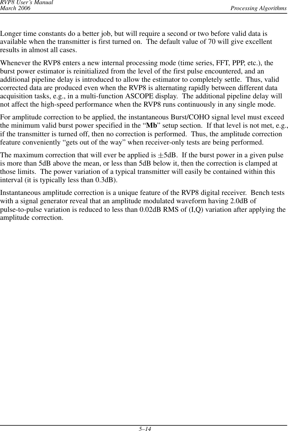
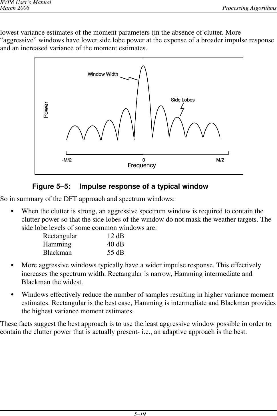
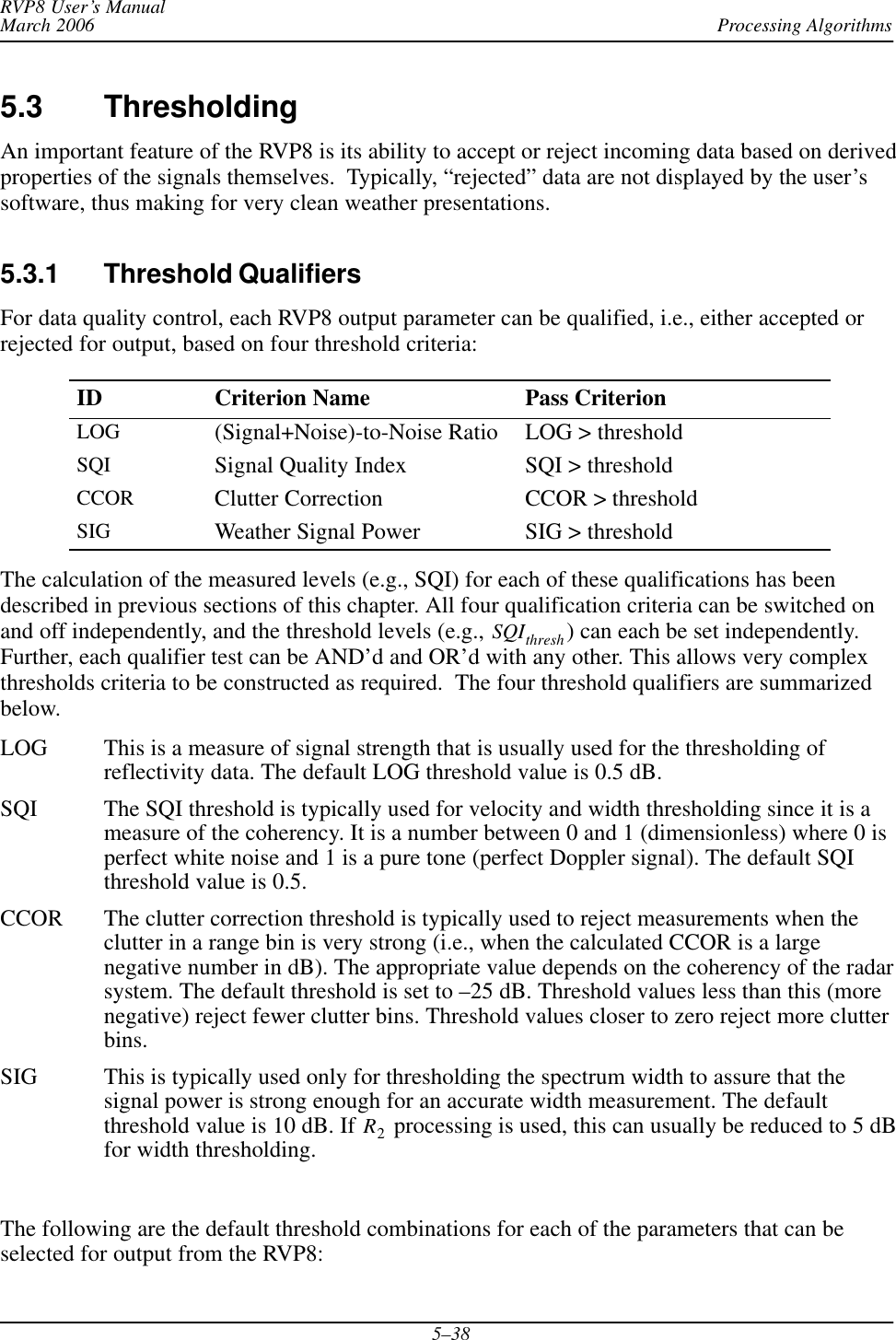
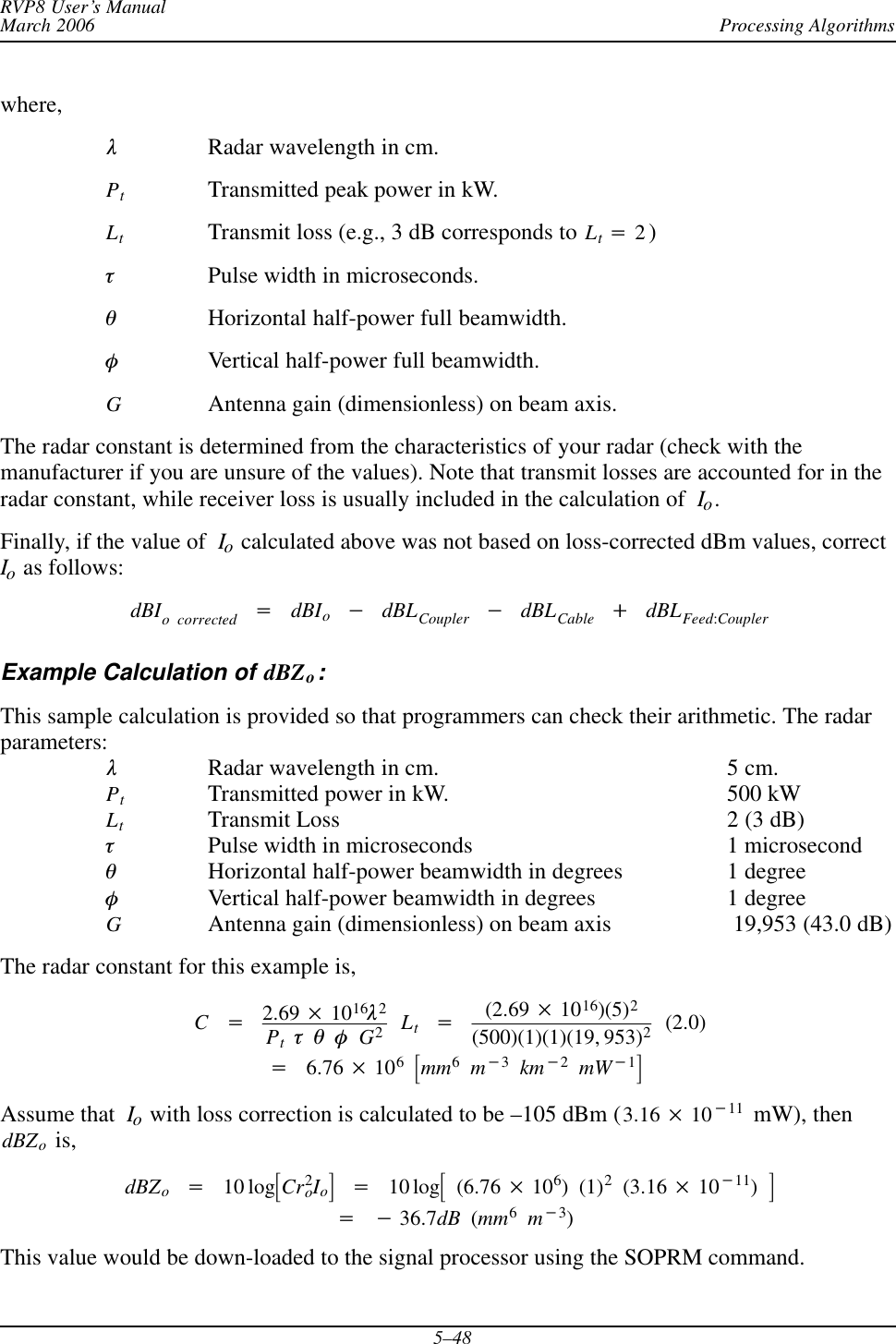
![Processing AlgorithmsRVP8 User’s ManualMarch 20065–345.2.8 VelocityFor a Doppler power spectrum that is symmetric about its mean velocity, the velocity is obtaineddirectly from the argument of the autocorrelation at the first lag, i.e.,V+l4ptsq1 where q1+arg NJR1Nj.l is the radar wavelength, ts is the sampling time (1/PRF). q1 is constrained to be on theinterval [*p,p]. When q1+" p , then V+" Vu where the unambiguous velocity is ,Vu+l4ts .If the absolute value of the true velocity of the scatterers is greater than Vu , then the velocitycalculated by the RVP8 is folded into the interval ƪ*Vu,Vuƫ , which is called the Nyquistinterval. Folding is usually easily recognized on a color display by a discontinuous jump invelocities. For example, if the true velocity is Vu)DV, then the velocity calculated by theRVP8 is *Vu)DV, which is 2Vu away from the true mean velocity.For 8-bit outputs, rather than calculating the absolute velocity in scientific units, the RVP8calculates the mean velocity for the normalized Nyquist interval [–1,1], i.e., the output valuesare,VȀ+q1p.For example, an output value of –0.5 corresponds to a mean velocity of *Vuń2. Thenormalized velocity VȀ is more efficient use of the limited number of bits.5.2.9 Spectrum Width AlgorithmsThe spectrum width is a measure of the combined effects of shear and turbulence. To a lesserextent, the antenna rotation rate can also effect the spectrum width. At high elevation angles, thefall speed dispersion of the scatterers also effects spectrum width.There are two choices for the spectrum width algorithm used in the RVP8, depending on thespeed and accuracy that are required for the application:R0,R1 “fast” algorithm valid when SNR >> 10 dBR0,R1,R2 “accurate” algorithm for SNR >> 0 to 5 dBThe approach used is selected in the SOPRM command. The two approaches are described below:R0,R1Width AlgorithmGiven samples of the Doppler autocorrelation function, numerous estimates of spectral vari-ance can be computed (Passarelli & Siggia, 1983). The particular estimator used by theRVP8 employs the magnitudes of R0 and R1 and assumes that the Doppler spectrum isGaussian (usually an acceptable assumption) and that the signal-to-noise ratio is large. Spe-cifically we have (similar to Srivastava, et al 1979):Variance +2lnƪRo|R1|ƫ+*2ln[SQI]](https://usermanual.wiki/Baron-Services/DSSR-250C.Processing-Algorithms/User-Guide-669147-Page-34.png)
![Processing AlgorithmsRVP8 User’s ManualMarch 20065–35where “ln” represents the natural logarithm. This can be compared to the expression in thepreceding section for SQI to illustrate that this expression for the variance is only valid when:SNRSNR )1[1which occurs when the SNR is large.This variance estimator is normalized to the Nyquist interval in units of [*p,p]. Thus, forexample, a variance of p2ń25 would be obtained from a Gaussian spectrum having a stan-dard deviation equal to one fifth of the total width of the plotted spectral distribution. Forscientific purposes, the spectrum width (standard deviation) is more physically meaningfulthan the variance, since it scales linearly with the severity of wind shear and turbulence. Forthese reasons, the width W is output by the RVP8:W+VarianceǸpAgain, for efficient packing in 8-bits, width is normalized to the Nyquist interval [–1, 1 ].For the example given above, the output width W would be (1/5). To obtain the width in me-ters per second, one multiplies the output width by Vu .R0,R1,R2 Width AlgorithmThe width algorithm in this case is similar except that the addition of R2 extends the validityof the width estimates to weak signals. In this case the variance is:Variance +23lnƪ|R1||R2|ƫThe output width W is then defined as in the previous section.5.2.10 Signal Quality Index (SQI threshold) An important feature of the RVP8 is its ability to eliminate signals which are either too weak tobe useful, or which have widths too large to justify further analysis. This is done via the signalquality index (SQI) which is defined as:SQI +|R1|R0The SQI is the normalized magnitude of the autocorrelation at lag 1 and varies between 0 for anuncorrelated signal (white noise) to 1 for a noise-free zero-width signal (pure tone). Meanvelocity estimates are degraded when the spectrum, width is large or when the signal-to-noiseratio is weak. The SQI is a good measure of the uncertainty in the velocity estimates and is aconvenient screening parameter to compute. In terms of the Gaussian model, the SQI is :SQI +SNRSNR )1e*p2W22where the SNR is the signal-to-noise ratio. For very large SNR’s the SQI is a function of thespectrum width only. For a zero-width pure tone (W=0), the SQI is a function of the SNR only(e.g., for W=0, an SNR of 1 corresponds to SQI=0.5). The SQI threshold is typically set to avalue of 0.4 to 0.5.](https://usermanual.wiki/Baron-Services/DSSR-250C.Processing-Algorithms/User-Guide-669147-Page-35.png)
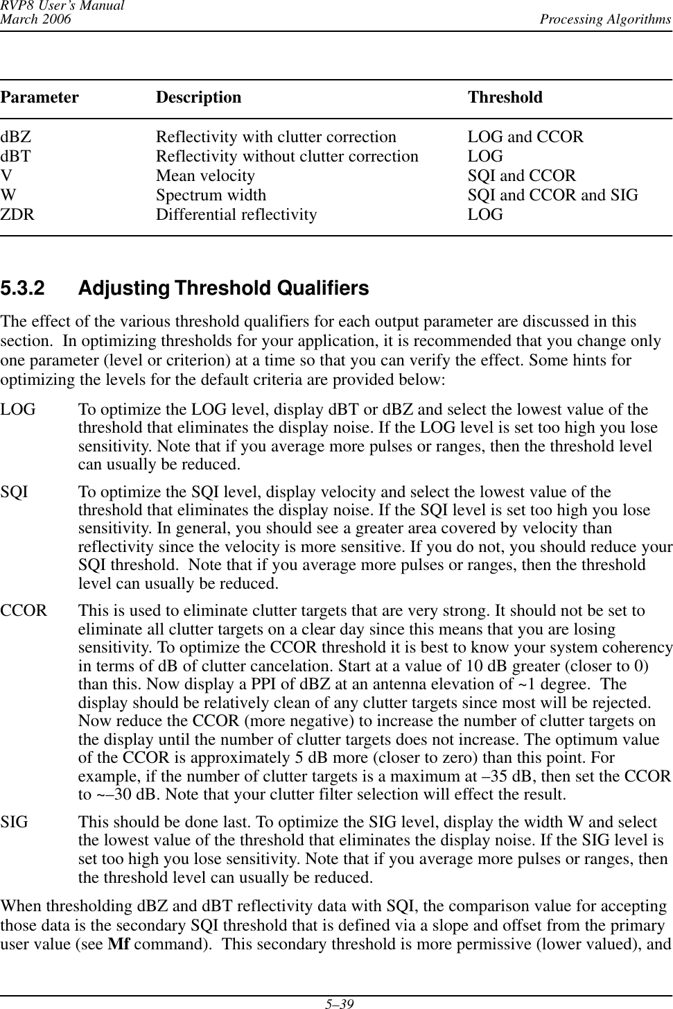
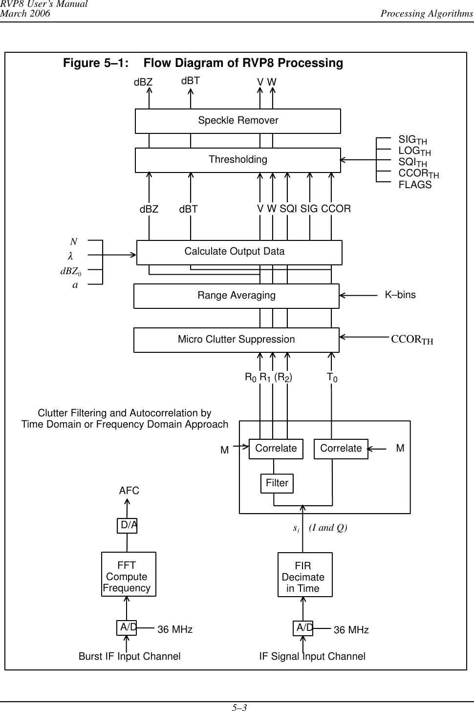
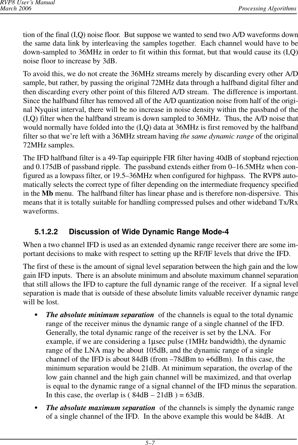
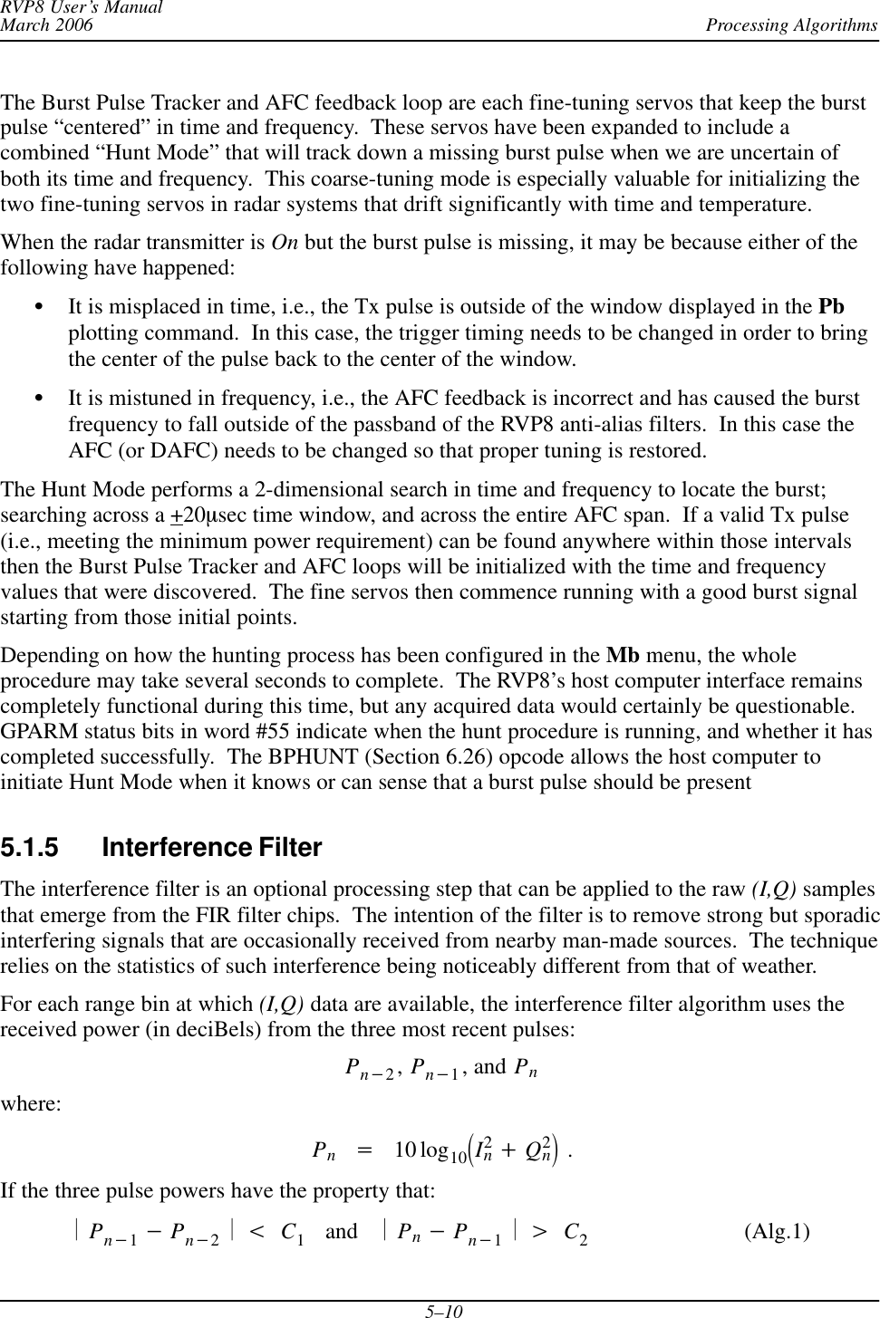
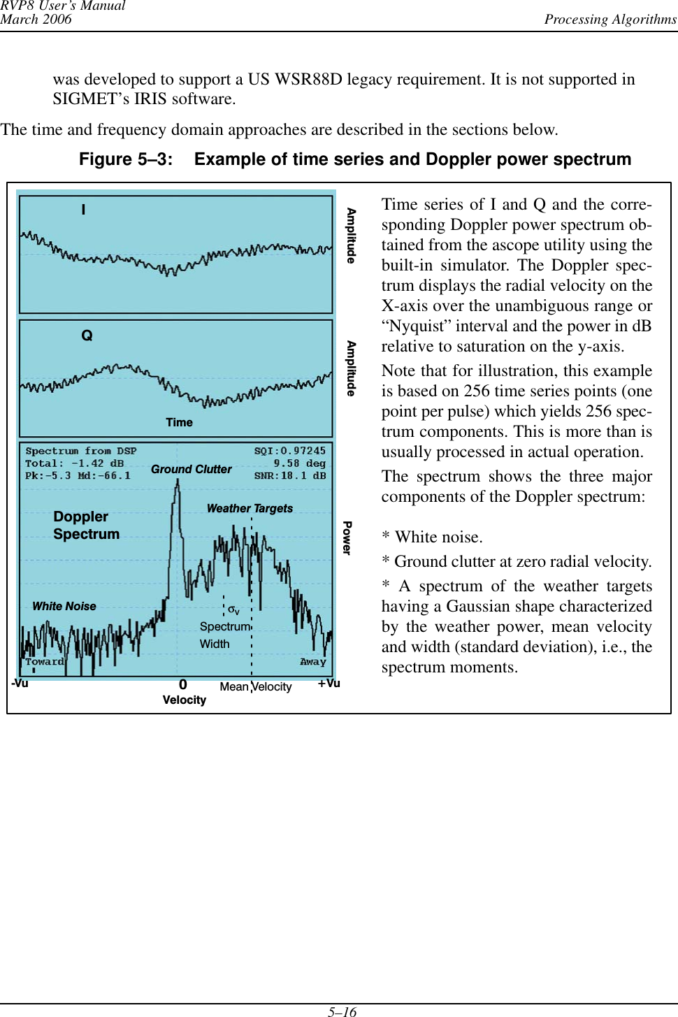
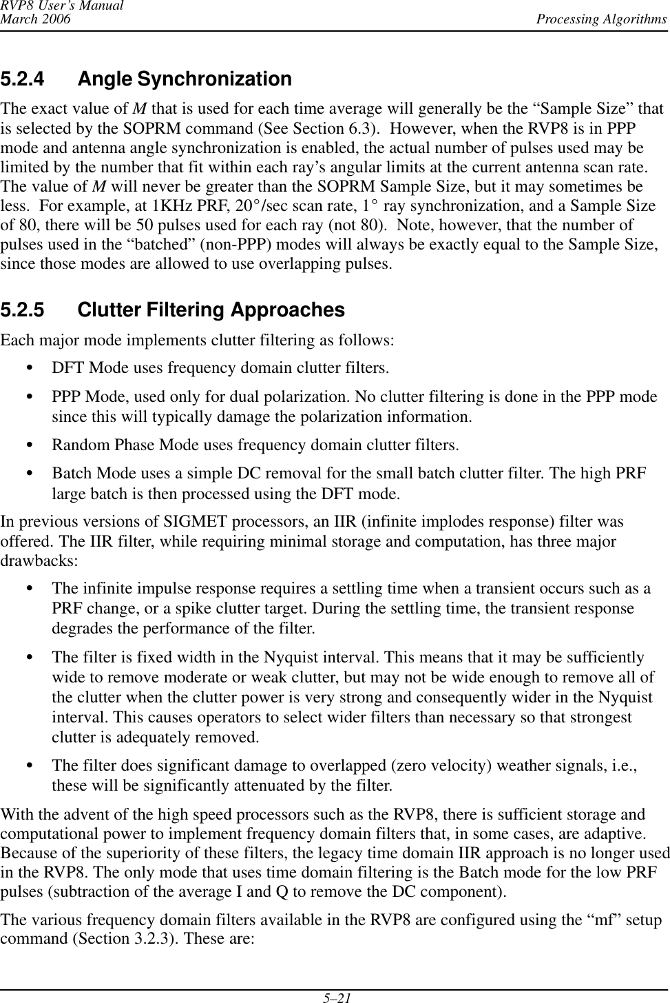
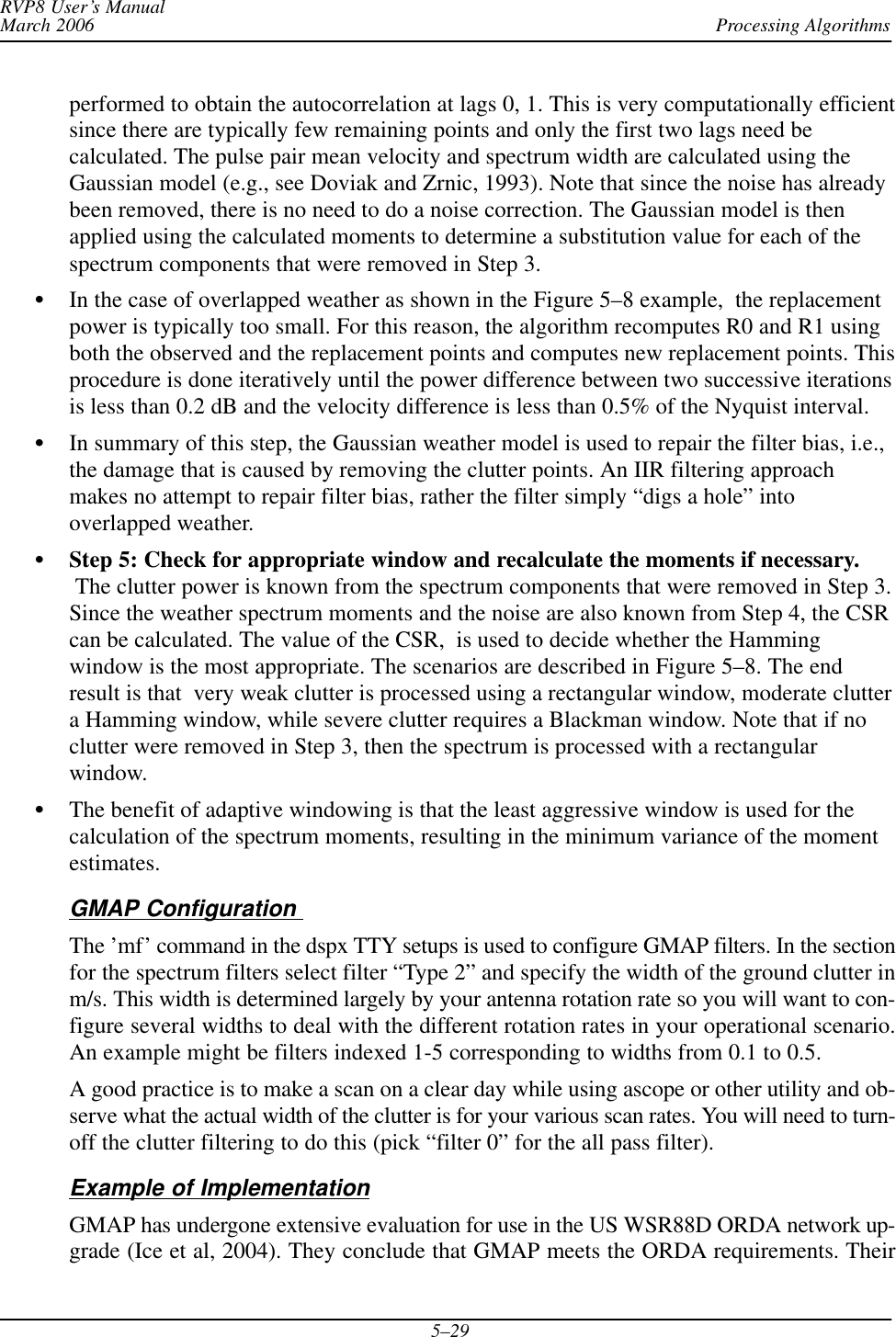
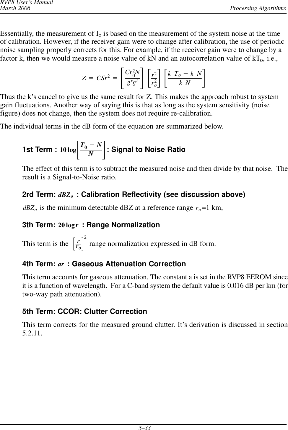
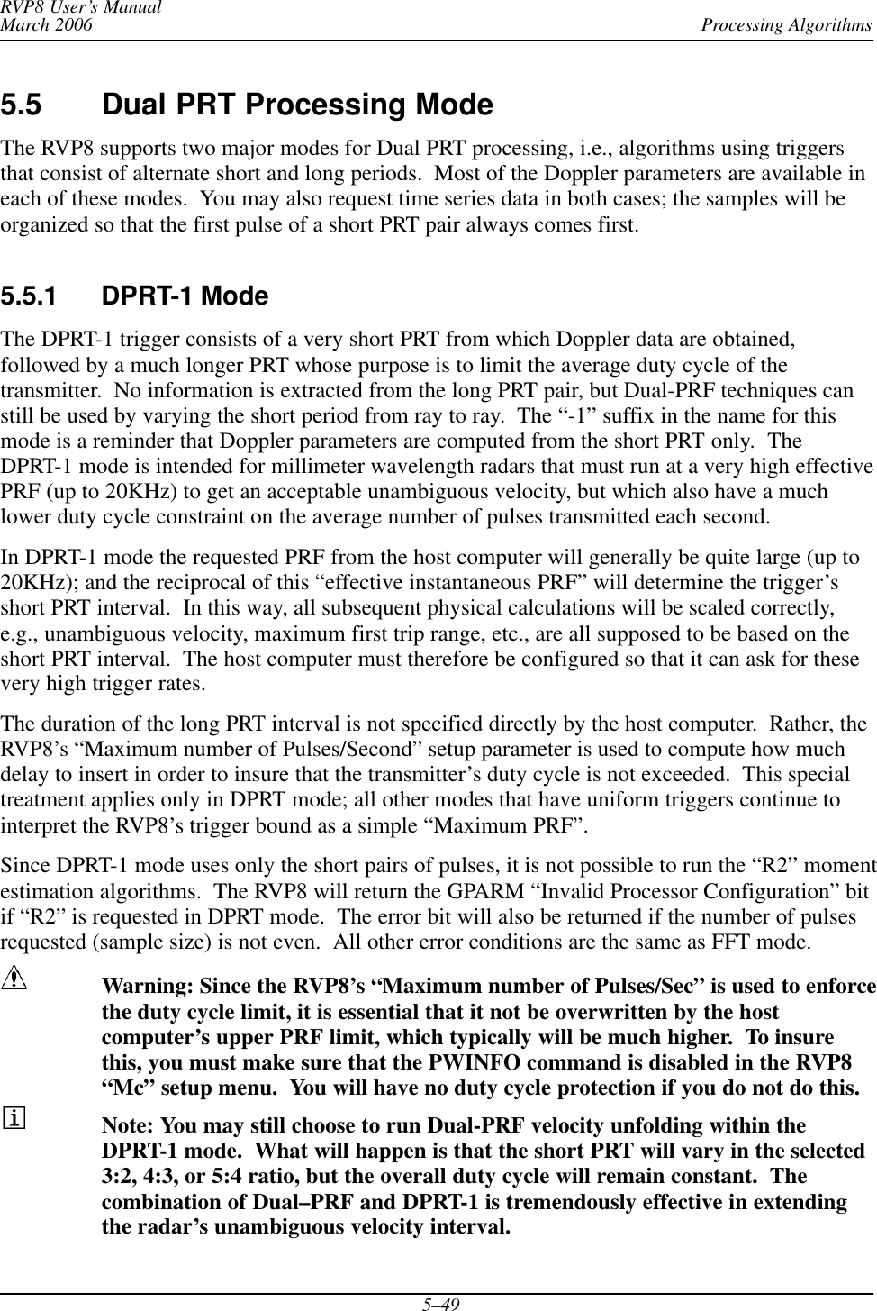
![Processing AlgorithmsRVP8 User’s ManualMarch 20065–42RangeAzimuth0-1101-1Zoutput00 +ThresholdThreshold if center point is valid but there are no or only one valid neighbor.Z00Z0*1RangeAzimuth0-1101-1Fill thresholded center point with average if there 6 or more valid neighbors.Z0*1Z*11 Z01Zoutput00 +[Z*11 )Z01 )Z11 )Z10 )Z*1*1)Z0*1]6RangeAzimuth00-11-12D Velocity Unfolding Step 1: Search pattern for valid second velocityPRF2PRF1V200231V11*1Z11Z10Z*1*1Indicates Thresholded Bin2D 3x3 Filtering ConceptsSStep 2: The unfolded velocities are then subjected to the standard 3x3 filtering.Dual PRF, Random Phase ProcessingIn random phase processing, the “seam” at the start of the second trip is always problematicsince the transmitter main bang and nearby clutter will virtually always wipe out the first few2nd trip range bins. At a constant PRF the 2nd trip seam is always at the same range, but indual PRF random phase mode, the seam is different each ray. Thus thresholded bins at theseam of the high PRF can be surrounded on either side by valid bins taken at the low PRF.The 3x3 filter has the effect of interpolating the reflectivity and width data over the bins atthe 2nd trip seam. Velocity data will also be filled–in using the nearest neighbor. Thus the](https://usermanual.wiki/Baron-Services/DSSR-250C.Processing-Algorithms/User-Guide-669147-Page-42.png)
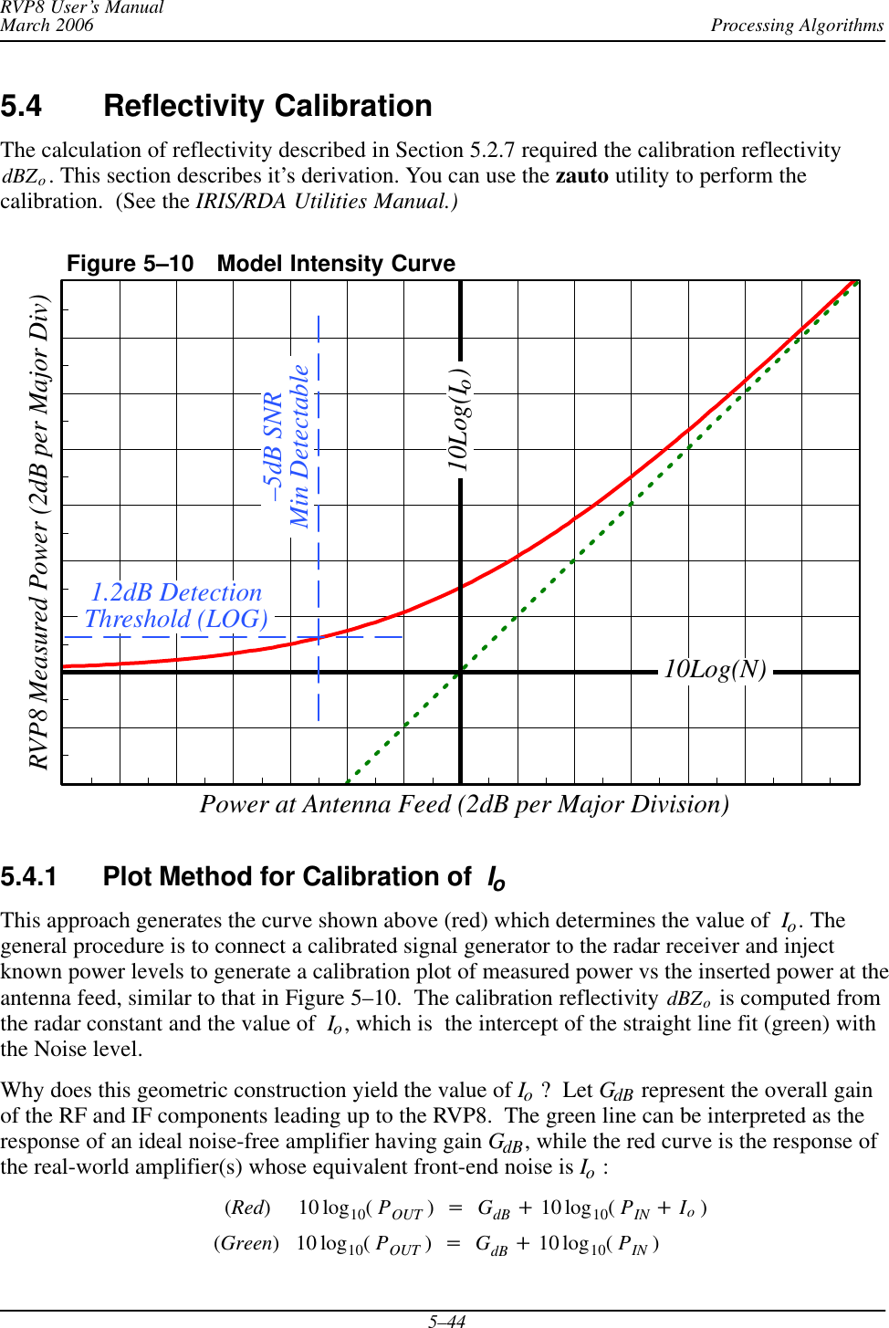
![Processing AlgorithmsRVP8 User’s ManualMarch 20065–46STurn the radiate off and connect the signal generator to the test signal injection point.SRaise the antenna to at least 20 degrees, and set the azimuth to point away from anyknown RF sources including the sun.SSelect the pulse width using the mt command.SSelect the pr command and use the commands to set the following: Plotting Received Power Spectrum... Rx:Pri, Zoom:x1–x8, Navg:25, Start:100.01 usec (14.99 km), Span:50 usecSSet the signal generator to the approximate radar RF frequency with a power levelcorresponding to a strong signal (30 dB above the noise), and use a CW signal (not apulse). This signal should be visible as a peak in the spectrum display. Adjust the siggenRF signal frequency so that produces the precise IF frequency (e.g., IF frequency of 30MHz).STurn the signal generator off and record the “Filtered” power level. Note that because ofthe large averaging it will require several seconds for the average to stabilize.STurn the signal generator on, verify that the peak is still at the IF frequency and adjustthe power level to obtain precisely 3 dB more “Filtered” power than was observed withthe noise only. Again, allow several seconds for the averaging to stabilize after you makeeach amplitude adjustment.This is the value of Io, i.e., the test signal signal power equals the noise power. The next step isto correct the value of Io for losses as discussed in the section below.5.4.3 Treatment of Losses in the CalibrationIn the calibration of the dBm level of the test signal, be sure to account for any losses that mayoccur between the antenna feed and the injection point, and in the cable and coupler that is usedto connect the signal generator to the injection point. Figure 5–11 illustrates the nomenclature ofthe various losses that are involved in the calibration. The relationship between the injected testsignal and the value of the received power relative to the feed is:dBmFeed +dBmInjected )dBLFeed:CouplerdBmFeed +dBmSiggen *dBLCoupler *dBLCable )dBLFeed:CouplerFor example, assume the following:Loss between the feed and the coupler dBLFeed:Coupler 3 dBLoss caused by the coupler dBLCoupler 30 dBLoss in the cable from siggen to coupler dBLCable 2 dBThen if the test signal generator output is –50 dBm, the injected power isdBmInjected = –50–[30+2]= –82 dBm.](https://usermanual.wiki/Baron-Services/DSSR-250C.Processing-Algorithms/User-Guide-669147-Page-46.png)
![Processing AlgorithmsRVP8 User’s ManualMarch 20065–515.6 Dual PRF Velocity UnfoldingFor a radar of wavelength l operating at a fixed sampling period ts+1ńPRF , the unambiguousvelocity and range intervals are given by:Vu+l4ts and Ru+cts2where “c” is the speed of light. Often these intervals do not fully cover the span of velocity andrange that one would like to measure. The problem is generally worse for short wavelengthradars, since that unambiguous velocity span is directly proportional to l for a given ts. If theunambiguous range interval is made sufficiently large by increasing ts , then the resultingvelocity span may be unacceptably small.The RVP8 provides a built-in mechanism for extending the unambiguous velocity span by afactor of two, three, or four beyond that given above. The technique, called Dual PRF velocityunfolding, uses two pulse periods rather than one, and relies on the extra information thusobtained to correct (i.e. unfold) the mean velocity measurement from each individual period.The Dual PRF trigger pattern consists of alternating (N+k)-pulse intervals where the period ineach interval is either tl (for the low-PRF) or th (for the high-PRF). Here “N” is the samplesize, and “k” represents a delay that permits the clutter filter to equilibrate to the new PRF aftereach change. The clutter filter impulse response lengths vary according to which filter isselected.The two trigger periods tl and th must be chosen in either a 3:2, 4:3, or 5:4 ratio. These ratiosgive factors of two, three, and four times velocity expansion over the th period alone. Theunfolding algorithm makes use of the following results. Suppose that the radar observes a targetwith mean velocity V at each of the two trigger periods. The measured phase angles for the R1autocorrelations at the two PRFs are:ql+4pVtll and qh+4pVthlwhere angles outside the basic [*p,p] interval are returned to that interval by appropriateadditions of "2p. These angles correspond to the ordinary single-PRF Doppler velocitymeasurements, and the "2p uncertainties reflects the fact that each measurement is foldedinto its own unambiguous interval:Vul +l4tl and Vuh +l4thIf we define f to be the difference between the two measured phases then:f+ql*qh+4plƪtl*thƫwhich can be interpreted as a phase angle within the unfolded interval:Vu unfold +l4(tl*th)](https://usermanual.wiki/Baron-Services/DSSR-250C.Processing-Algorithms/User-Guide-669147-Page-51.png)
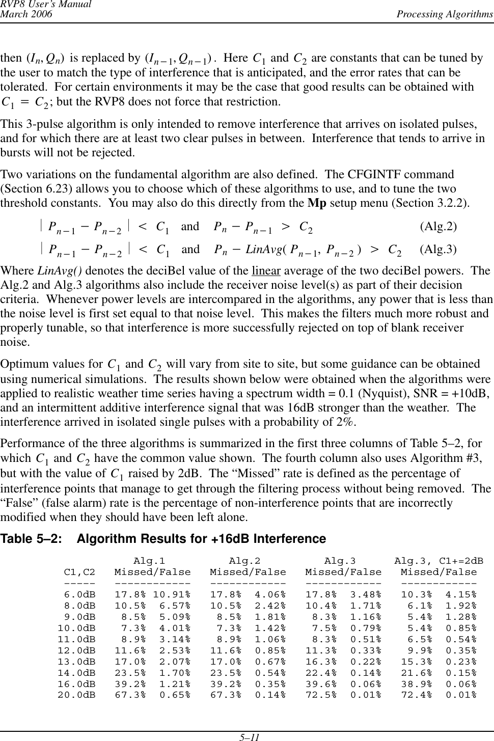
![Processing AlgorithmsRVP8 User’s ManualMarch 20065–52Now if tl and figureth are in a 3:2 ratio, then:tl*th+tl3+th2and thus Vu unfold +3Vul +2VuhThe angle f represents a velocity phase angle in [*p,p] , but with respect to an enlargedunambiguous interval. Thus, by simply differencing the folded angles from the high and lowPRFs, we obtain an angle that is unfolded to a larger velocity span. Similar reasoning shows thatthe 4:3 ratio gives a factor of three improvement over Vuh , and 5:4 gives a factor of four.In practice, the unfolded angle f is not in itself a suitable velocity estimator. The reason is thatthe variance of f is equal to the sum of the variances of each of its components, i.e., twice thatof the individual measurements alone. If the target is at all noisy, then this increase in variancecan be severe. Rather than use f directly, the RVP8 uses it only as a rough estimate indetermining how to unfold the individual velocity measured from each PRF.Figure 5–12: Dual PRF Conceptsql*qhResultqlń3Region IIIRegion IIRegion ILow PRF Case High PRF CaseRegion IRegion IIql*qhResultqhń2This technique is illustrated in Figure 5–12. The figure shows how the low-PRF and high-PRFangles are unfolded based on the difference angle. The diagrams show phase planes representingthe large unfolded velocity interval, and the locations of various vectors on those planes.Referring first to the right figure, the difference angle is plotted, and the plane is divided intotwo equal size regions, one of which is centered on the difference vector. The high-PRF angle isthen divided by two and plotted. The resultant unfolded velocity angle must either be this vector,or this vector plus p. Since adding p places the vector into acceptance Region 1 where it is](https://usermanual.wiki/Baron-Services/DSSR-250C.Processing-Algorithms/User-Guide-669147-Page-52.png)
![Processing AlgorithmsRVP8 User’s ManualMarch 20065–53nearest the difference angle, we conclude that this is the correct unfolding. Likewise, on the leftdiagram we unfold the low-PRF angle by dividing the plane into thirds centered on thedifference angle. The result angle is eitherql3,ql3)2p3or ql3)4p3depending on which one falls into the acceptance Region 1. Note that the resultant angle is thesame in each case.The RVP8 makes efficient use of the incoming data by unfolding velocities from both the lowand the high-PRF data, making use each time of information in the previous ray. When low-PRFdata are taken the derived velocities are unfolded by combining information from the previoushigh-PRF interval. Likewise, when high-PRF data are acquired the velocities are unfolded basedon the previous low-PRF interval. Thus, when operating in the Dual PRF mode, the RVP8outputs one data ray for each (N+k)-pulse interval. However, the velocity data in the Dual PRFrays are unfolded, so that the [–1,+1] interval now represents either two or three times the priorvelocity range. Put another way, the data are still interpreted as described in the section on meanvelocity estimation, except that Vu is now larger.The width data are also modified somewhat during Dual PRF unfolding. Although valid widthsare obtained independently on all rays, those measured at low-PRF are larger than those athigh-PRF. This is simply because the dimensionless width units are with respect to a largervelocity interval in the latter case. To compensate for this, low-PRF widths are multiplied byeither 2/3 or 3/4 before being output. This puts them in the same scale as the high-PRF values,and thus, the widths do not vary on alternate pulses. A useful consequence of this is that widthdata can be sent directly to a color display generator without having to plot every other ray in adifferent scale.There are a few words of caution that should be kept in mind when using the RVP8 in the DualPRF processing modes. The unfolding algorithms make the assumption that targets aremore-or-less continuous from ray to ray. Otherwise, it would not make sense to use data from aprevious ray to unfold velocities in the current ray. Users must therefore assure that their antennascan rate and beamwidth are such that each target is illuminated, at least partially, over each full2(N+k)-pulse interval. In practice, a certain amount of decorrelation from ray to ray isacceptable, since the previous rays are used only to decide into which unfolded interval thecurrent ray should be placed. Small errors in the previous ray data, therefore, cause no error inthe output. However, large previous-ray errors would lead to incorrect unfolding.A more subtle side effect of Dual PRF processing arises from clutter filtering because clutternotches now appear at several locations in the unfolded velocity span, rather than just at zerovelocity. These additional rejection points come about because the original velocity intervals aremapped some integer number of times to create the unfolded interval. Since each originalinterval has a clutter notch at DC, it follows that the final expanded velocity interval will haveseveral such notches. For example, in the 3:2 case, in addition to removing DC the clutter filterremoves velocities at *2Vuń3,)2Vuń3, and Vu.Unfortunately, these clutter filter “images” are a fundamental consequence of the Dual PRFprocessing technique and are not easily removed. They can cause trouble not only for thevelocity unfolding itself, but because the computed clutter corrections to be wrong at the image](https://usermanual.wiki/Baron-Services/DSSR-250C.Processing-Algorithms/User-Guide-669147-Page-53.png)