Baron Services DSSR-250C Pulsar Digital Solid-State Radar System User Manual
Baron Services Inc Pulsar Digital Solid-State Radar System
UserManual.wiki
>
Baron Services
>
DSSR-250C User Manual
>
Plot Assisted Setups
Contents
1.
Users Manaul Cover Page and Table of Contents
2.
Hardware Limited Warranty
3.
Introduction and Specifications
4.
Hardware Installation
5.
Plot Assisted Setups
6.
Processing Algorithms
7.
TTY Nonvolatile Setups
8.
Host Computer Commands
Plot Assisted Setups
Navigation menu
Upload a User Manual
Namespaces
Wiki Guide
HTML
PDF
Info
Views
User Manual
Discussion / Help
Navigation
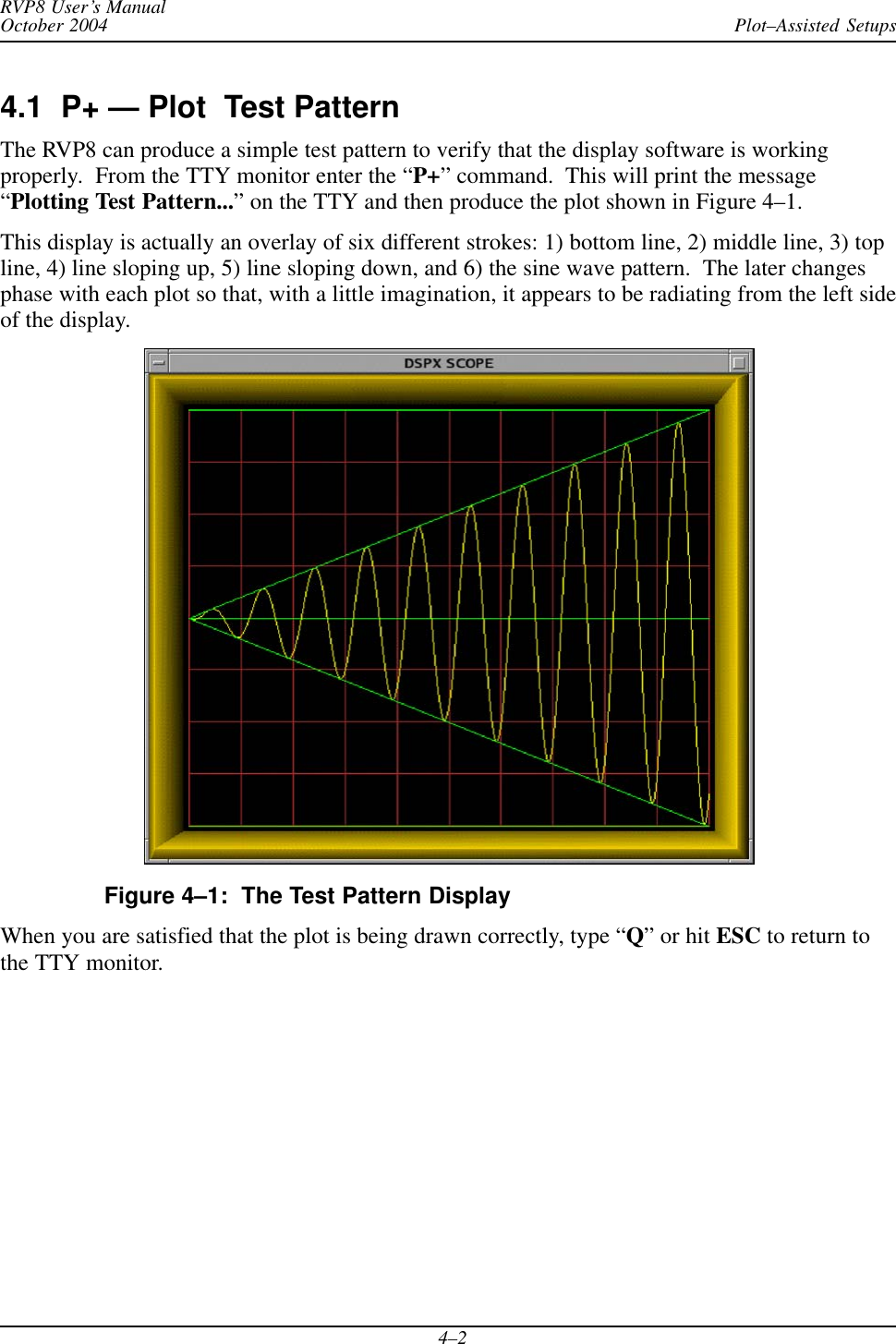
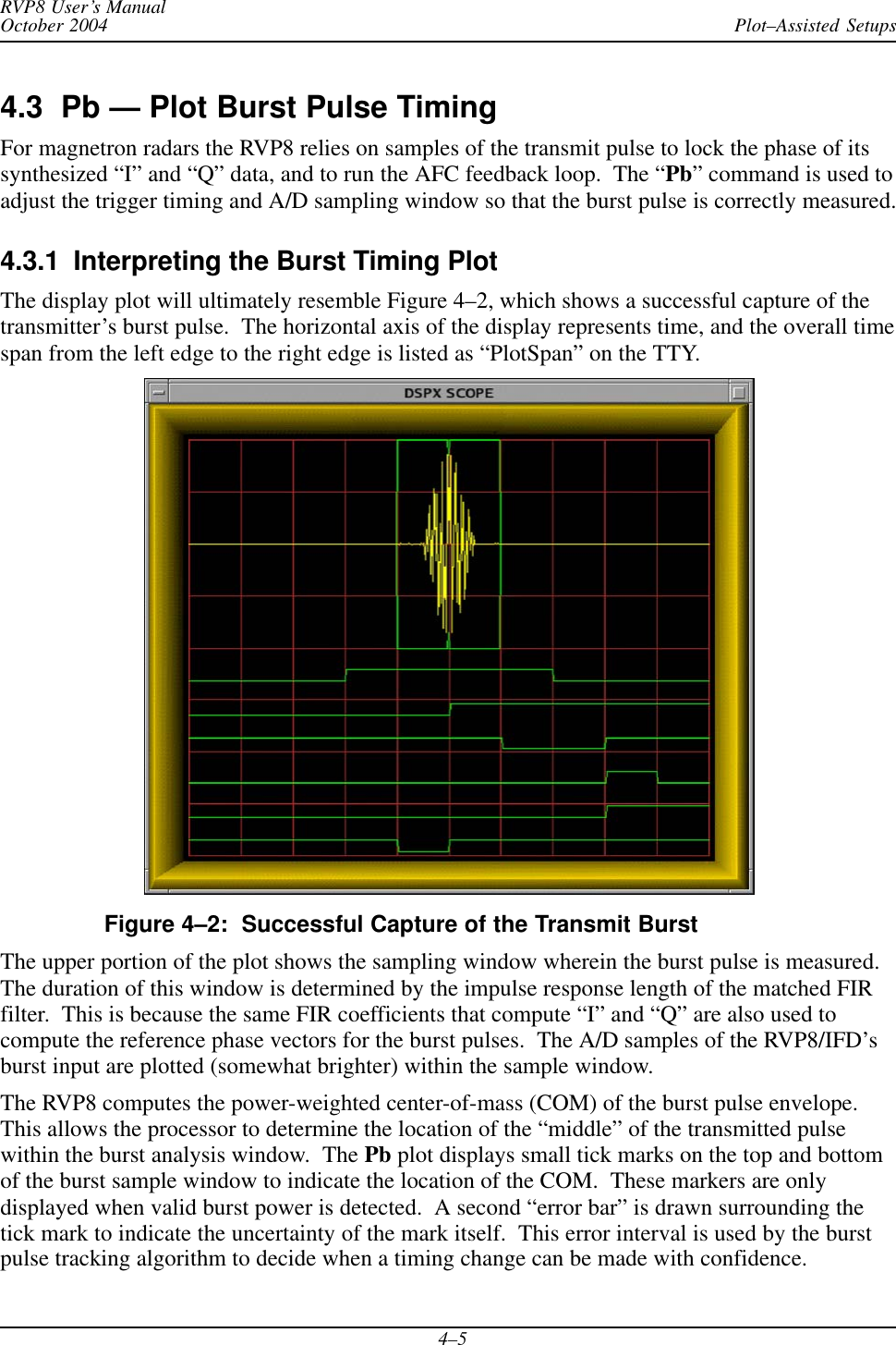
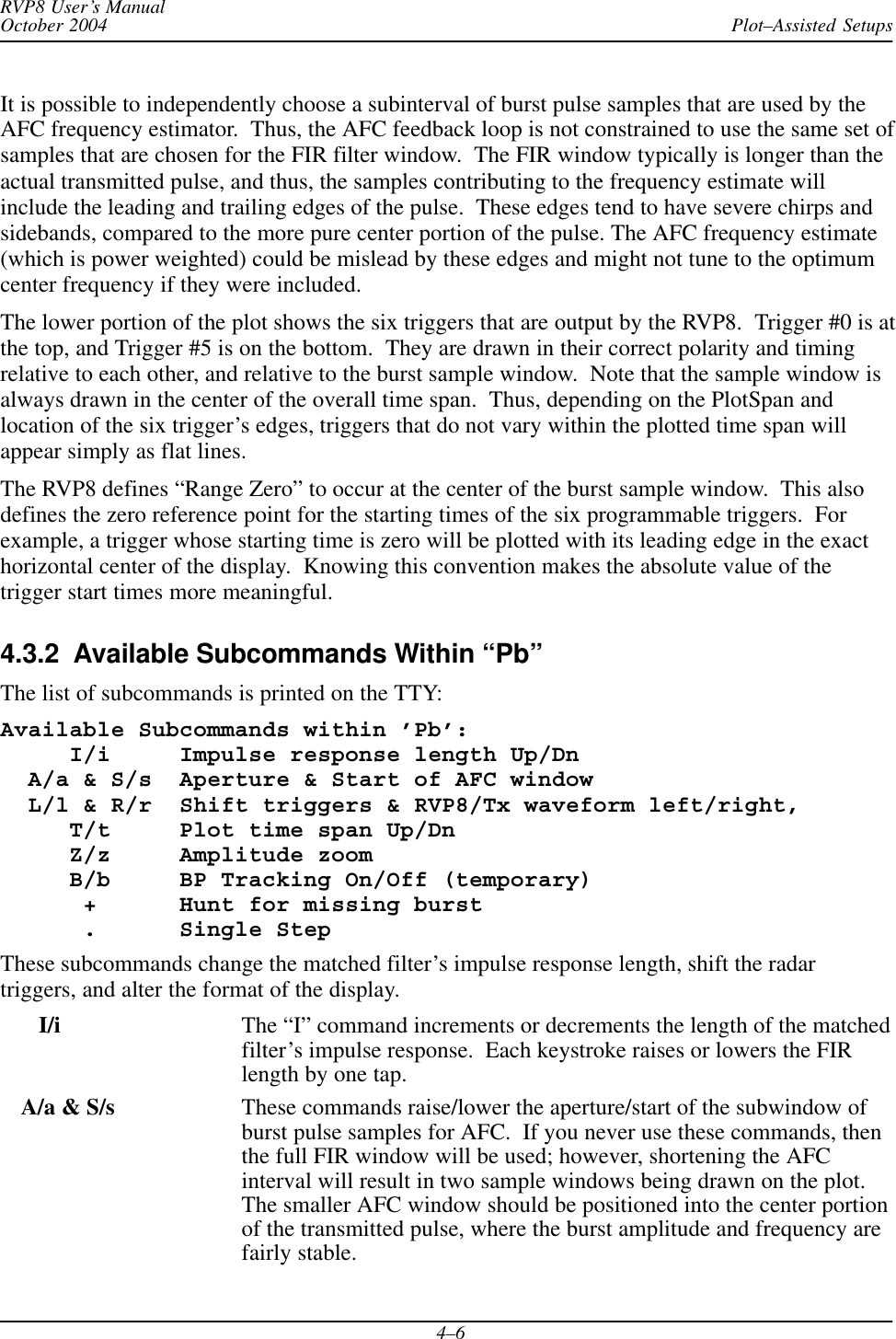
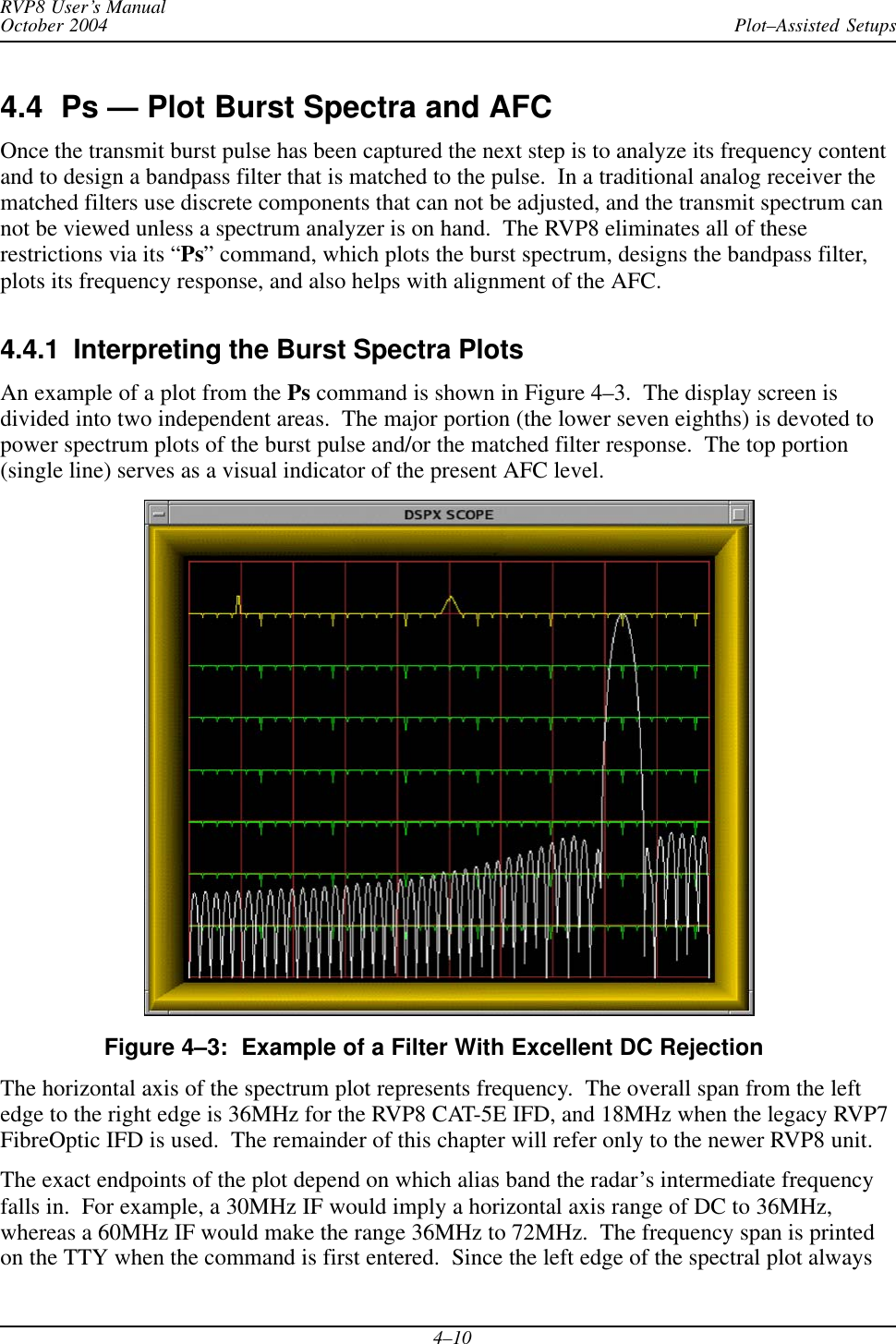
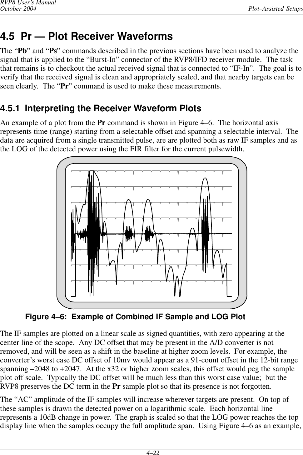
![Plot–Assisted SetupsRVP8 User’s ManualOctober 20044–30Z/z The dynamic range of the Pa sidelobe plot is 80dB. Usually this willgive plenty of room to examine the properties of the waveform. Butfor very wide dynamic range pulses, you can shift the plot up/down in10dB steps using these “Zoom” keys.$Designs an optimal compressed waveform. For a given pulsewidthand bandwidth of the Tx waveform, this command allows you to trymany thousands of combinations of FM shape and amplitude shape,searching for the one that minimizes the sum of PSL and ISL (in dB).This gives the best overall waveform for weather radar observations inwhich both the PSL and ISL are important.The following dialog appears in response to the “$” command: TuningParam #1 (0.9000) –– 1 Grid Point from 0.9000 to 0.9000 TuningParam #2 (1.0000) –– 1 Grid Point from 1.0000 to 1.0000 TuningParam #3 (0.1774) –– 1 Grid Point from 0.1774 to 0.1774As the line is printed for each parameter, you may either accept thedefault single grid point (no search), or enter a desired number of gridsearch points followed by a span of values within which to search.For example, typing:200 .9 .95will request that the parameter be searched using 200 evenly spacedgrid points lying between 0.9000 and 0.9500 inclusive. After all threeparameter spans have been entered, the RVP8 will begin searching forthe optimum waveform. Progress messages are printed on the TTY,and the plot will update every time a better waveform is discovered.In this way it is easy to tell whether the search is converging.The process normally runs to completion on its own; but if the searchis taking too long, or you’ve changed your mind about which intervalsto search, typing “Q” will exit right away. In either case, the prompt:Keep this waveform ? [Y]will appear. Typing “Y” (or Enter) will keep the optimized tuningparameters that were just discovered, overwriting whatever startingvalues were originally there. Typing “N” will discard the searchresults and return to the original settings, as if “$” had never beentyped.4.6.3 TTY Information Lines Within “Pa”The TTY information lines will resemble:BW:3.40MHz PW:29.99usec PSL:–61.2dB ISL:–51.3dB TxLoss:0.5dB RxLoss:2.4dBBW Bandwidth of the Tx waveform in MegaHertz.PW Pulsewidth (pulse length) of the Tx waveform in microseconds.](https://usermanual.wiki/Baron-Services/DSSR-250C.Plot-Assisted-Setups/User-Guide-669146-Page-30.png)